# TensorFlow API
## 一、TensorFlow的API查阅
TensorFlow官方文档_w3cschool:
(1) 关于《TensorFlow官方文档》
《TensorFlow官方文档》原文地址:,本次经过 W3Cschool.cn 进行翻译整理,让大家能更好的认识机器学习。机器学习可能是未来新品和新技术的一个关键部分。
TensorFlow 是谷歌基于 DistBelief 进行研发的第二代人工智能学习系统,而谷歌的工程师们也正在使用TensorFlow 作为内部的机器学习系统。现在,谷歌已经将其开源,并将他们使用 TensorFlow 的效果分享在许多的科研文章中。
机器学习行业的发展速度很快,为了能够让更多技术人员有效的学习到这一先进的人工智能学习系统, W3Cschool 对 TensorFlow 官方文档进行中文翻译,其中有纰漏之处希望各位能够提出。
(2) 谁可以用 TensorFlow?
Tensorflow 是属于任何人的,不管你的身份是学生、研究员、工程师、开发者、创业者或者等等都可以在 Apache 2.0 开源协议下使用 Tensorflow,只要您对 Tensorflow 感兴趣。
(3) 一起了解TensorFlow
TensorFlow 是一个采用数据流图(data flow graphs),用于数值计算的开源软件库。节点(Nodes)在图中表示数学操作,图中的线(edges)则表示在节点间相互联系的多维数据数组,即张量(tensor)。它灵活的架构让你可以在多种平台上展开计算,例如台式计算机中的一个或多个CPU(或GPU),服务器,移动设备等等。TensorFlow 最初由 Google 大脑小组(隶属于 Google 机器智能研究机构)的研究员和工程师们开发出来,用于机器学习和深度神经网络方面的研究,但这个系统的通用性使其也可广泛用于其他计算领域。
## 二、TensorFlow常见API的使用
### (0) API查询索引
> *参考来源:CSDN博主 [zj360202的博文](https://blog.csdn.net/zj360202/article/details/70243424) + 网上其他博文资料*
### (1) tf.placeholder函数
`tf.placeholder(dtype, shape=None, name=None)`:此函数可以理解为形参,用于定义过程,在执行的时候再赋具体的值。
参数:
- dtype:数据类型。常用的是 tf.float32、tf.float64 等数值类型
- shape:数据形状。默认是 None,就是一维值,也可以是多维,比如 [2, 3]、[None, 3] 表示列是 3,行不定
- name:名称。
```python
x = tf.placeholder(tf.float32, shape=(1024, 1024))
y = tf.matmul(x, x)
with tf.Session() as sess:
print(sess.run(y)) # ERROR: 此处x还没有赋值.
rand_array = np.random.rand(1024, 1024)
print(sess.run(y, feed_dict={x: rand_array})) # Will succeed.
```
返回:Tensor 类型。
参考:[tf.placeholder函数](https://blog.csdn.net/zj360202/article/details/70243127)
### (2) tf.nn.conv2d是怎样实现卷积的
tf.nn.conv2d 是 TensorFlow 里面实现卷积的函数:`tf.nn.conv2d(input, filter, strides, padding, use_cudnn_on_gpu=None, name=None)`
除去 name 参数用以指定该操作的 name,与方法有关的一共五个参数:
- input:指需要做卷积的输入图像,它要求是一个 Tensor,具有`[batch, in_height, in_width, in_channels]`这样的 shape,具体含义是`[训练时一个batch的图片数量, 图片高度, 图片宽度, 图像通道数]`,注意这是一个 4 维的 Tensor,要求类型为 float32 和 float64 其中之一
- filter:相当于 CNN 中的卷积核,它要求是一个 Tensor,具有`[filter_height, filter_width, in_channels, out_channels]`这样的 shape,具体含义是`[卷积核的高度,卷积核的宽度,图像通道数,卷积核个数]`,要求类型与参数 input 相同,有一个地方需要注意,第三维 in_channels,就是参数 input 的第四维
- strides:卷积时在图像每一维的步长,这是一个一维的向量,长度4
- padding:string 类型的量,只能是"SAME","VALID"其中之一,这个值决定了不同的卷积方式(后面会介绍)就是VALID只能匹配内部像素;而SAME可以在图像外部补0,从而做到只要图像中的一个像素就可以和卷积核做卷积操作,而VALID不行
- use_cudnn_on_gpu:bool 类型,是否使用 cudnn 加速,默认为 true
参考:[tf.nn.conv2d是怎样实现卷积的?](https://blog.csdn.net/zj360202/article/details/70243424)
### (3) tf.nn.max_pool实现池化操作
max pooling 是 CNN 当中的最大值池化操作,其实用法和卷积很类似:`tf.nn.max_pool(value, ksize, strides, padding, name=None)`
参数是四个,和卷积很类似:
- value:需要池化的输入,一般池化层接在卷积层后面,所以输入通常是 feature map,依然是`[batch, height, width, channels]这样的shape`
- ksize:池化窗口的大小,取一个四维向量,一般是`[1, height, width, 1]`,因为我们不想在 batch 和 channels 上做池化,所以这两个维度设为了 1
- strides:和卷积类似,窗口在每一个维度上滑动的步长,一般也是`[1, stride,stride, 1]`
- padding:和卷积类似,可以取'VALID' 或者'SAME'
返回一个 Tensor,类型不变,shape 仍然是`[batch, height, width, channels]`这种形式。
参考:[tf.nn.max_pool实现池化操作](https://blog.csdn.net/zj360202/article/details/70243836)
### (4) tf.nn.relu函数
`tf.nn.relu(features, name=None)` = `max(0,features)`
参数:
- features:Tensor 类型
- name:名称
一般 features 会是(卷积核,图像)的卷积后加上 bias。如:
```python
tf.nn.relu(tf.nn.conv2d(x_image, w_conv1, strides=[1, 1, 1, 1], padding='SAME') + b_conv1)
```
参考:[tf.nn.relu函数](https://blog.csdn.net/zj360202/article/details/70256545)
### (5) tf.reshape、tf.get_shape和set_shape函数
`tf.reshape(tensor, shape, name=None)`:数据重定形状函数。
参数:
- tensor:输入数据
- shape:目标形状
- name:名称
返回:Tensor
tf.shape(a) 和 tf.get_shape(a) 的区别:
①相同点:都可以得到 tensor a 的尺寸
②不同点:
- tf.shape() 中 a 数据的类型可以是 tensor、list、array
- a.get_shape() 中 a 的数据类型只能是 tensor,且返回的是一个元组(tuple):返回的是 tensor 每个维度的大小。
```python
import tensorflow as tf
import numpy as np
x=tf.constant([[1,2,3],[4,5,6]]
y=[[1,2,3],[4,5,6]]
z=np.arange(24).reshape([2,3,4]))
sess=tf.Session()
# tf.shape()
x_shape=tf.shape(x) # x_shape 是一个tensor
y_shape=tf.shape(y) #
z_shape=tf.shape(z) #
print sess.run(x_shape) # 结果:[2 3]
print sess.run(y_shape) # 结果:[2 3]
print sess.run(z_shape) # 结果:[2 3 4]
#a.get_shape()
x_shape=x.get_shape() # (2, 3):返回的是TensorShape([Dimension(2), Dimension(3)]),不能使用 sess.run() 因为返回的不是tensor 或string,而是元组
x_shape=x.get_shape().as_list() # 可以使用 as_list()得到具体的尺寸,x_shape=[2 3]
y_shape=y.get_shape() # AttributeError: 'list' object has no attribute 'get_shape'
z_shape=z.get_shape() # AttributeError: 'numpy.ndarray' object has no attribute 'get_shape'
```
[TensorFlow的reshape操作 tf.reshape](https://blog.csdn.net/lxg0807/article/details/53021859)
tf.reshape(tensor, shape, name=None) 函数的作用是将 tensor 变换为参数 shape 的形式。
其中 shape 为一个列表形式,特殊的一点是列表中可以存在 -1。-1 代表的含义是不用我们自己指定这一维的大小,函数会自动计算,但列表中只能存在一个 -1。(当然如果存在多个 -1,就是一个存在多解的方程了)
好了我想说的重点还有一个就是根据shape如何变换矩阵。其实简单的想就是:
```shell
reshape(t, shape) => reshape(t, [-1]) => reshape(t, shape)
```
首先将矩阵 t 变为一维矩阵,然后再对矩阵的形式更改就可以了。
```python
# tensor 't' is [1, 2, 3, 4, 5, 6, 7, 8, 9]
# tensor 't' has shape [9]
reshape(t, [3, 3]) ==> [[1, 2, 3],
[4, 5, 6],
[7, 8, 9]]
# tensor 't' is [[[1, 1], [2, 2]],
# [[3, 3], [4, 4]]]
# tensor 't' has shape [2, 2, 2]
reshape(t, [2, 4]) ==> [[1, 1, 2, 2],
[3, 3, 4, 4]]
# tensor 't' is [[[1, 1, 1],
# [2, 2, 2]],
# [[3, 3, 3],
# [4, 4, 4]],
# [[5, 5, 5],
# [6, 6, 6]]]
# tensor 't' has shape [3, 2, 3]
# pass '[-1]' to flatten 't'
reshape(t, [-1]) ==> [1, 1, 1, 2, 2, 2, 3, 3, 3, 4, 4, 4, 5, 5, 5, 6, 6, 6]
# -1 can also be used to infer the shape
# -1 is inferred to be 9:
reshape(t, [2, -1]) ==> [[1, 1, 1, 2, 2, 2, 3, 3, 3],
[4, 4, 4, 5, 5, 5, 6, 6, 6]]
# -1 is inferred to be 2:
reshape(t, [-1, 9]) ==> [[1, 1, 1, 2, 2, 2, 3, 3, 3],
[4, 4, 4, 5, 5, 5, 6, 6, 6]]
# -1 is inferred to be 3:
reshape(t, [ 2, -1, 3]) ==> [[[1, 1, 1],
[2, 2, 2],
[3, 3, 3]],
[[4, 4, 4],
[5, 5, 5],
[6, 6, 6]]]
# tensor 't' is [7]
# shape `[]` reshapes to a scalar
reshape(t, []) ==> 7
```
[Tensorflow set_shape()和reshape()的区别](https://blog.csdn.net/oMoDao1/article/details/82079591)
这两个主要是适用场合的区别,前者用于更新图中某个 tensor 的 shape,而后者则往往用于动态地创建一个新的 tensor。
set_shape 的典型用法如下:
```python
import tensorflow as tf
x1 = tf.placeholder(tf.int32)
x1.set_shape([2, 2])
print(x1.get_shape())
sess = tf.Session()
#print(sess.run(tf.shape(x1), feed_dict={x1:[0,1,2,3]}))
print(sess.run(tf.shape(x1), feed_dict={x1:[[0,1],[2,3]]}))
```
输出:
```python
(2, 2)
[2 2]
```
这代表了图中最开始没有 shape 的 x1 在使用了 set_shape 后,它的图中的信息已经改变了,如果取消掉注释就会报错,因为我们传入了和图不符合的参数。
### (6) tf.nn.dropout函数
`tf.nn.dropout(x, keep_prob, noise_shape=None, seed=None, name=None)`:此函数是为了防止在训练中过拟合的操作,将训练输出按一定规则进行变换。
- x:输入
- keep_prob:保留比例。取值 (0, 1] ,每一个参数都将按这个比例随机变更。
- noise_shape:干扰形状。此字段默认是 None,表示第一个元素的操作都是独立,但是也不一定。比例:数据的形状是 shape(x)=[k, l, m, n],而 noise_shape=[k, 1, 1, n],则第 1 和 4 列是独立保留或删除,第 2 和 3 列是要么全部保留,要么全部删除。
- seed:了解不多
- name
返回:Tensor
```python
tf.nn.dropout(20,0.8)
```
### (7) tf.argmax函数
`tf.argmax(input, axis=None, name=None, dimension=None)`:此函数是对矩阵按行或列计算最大值。
参数:
- input:输入Tensor
- axis:0 表示按列,1 表示按行
- name:名称
- dimension:和 axis 功能一样,默认 axis 取值优先。新加的字段。
返回:Tensor,一般是行或列的最大值下标向量
```python
import tensorflow as tf
a=tf.get_variable(name='a',
shape=[3,4],
dtype=tf.float32,
initializer=tf.random_uniform_initializer(minval=-1,maxval=1))
b=tf.argmax(input=a,axis=0)
c=tf.argmax(input=a,dimension=1) #此处用dimesion或用axis是一样的
sess = tf.InteractiveSession()
sess.run(tf.initialize_all_variables())
print(sess.run(a))
#[[ 0.04261756 -0.34297419 -0.87816691 -0.15430689]
# [ 0.18663144 0.86972666 -0.06103253 0.38307118]
# [ 0.84588599 -0.45432305 -0.39736366 0.38526249]]
print(sess.run(b))
#[2 1 1 2]
print(sess.run(c))
#[0 1 0]
```
参考:[tf.argmax函数](https://blog.csdn.net/zj360202/article/details/70259999)
另外也会看到有的代码中写到:axis = -2、-1,究竟是什么含义呢?参考该文:[Numpy、TensorFlow和Keras函数输入参数axis理解](https://blog.csdn.net/zenghaitao0128/article/details/78905593)
沿着指定 axis 轴的方向寻找最大值,并返回对应的索引。
```python
import numpy as np
import tensorflow as tf
A = np.random.random((3,4))
x = tf.constant(A)
sess = tf.InteractiveSession()
print("输入张量:\n",x.eval())
y1 = tf.argmax(x)
print("axis缺省时,默认axis = 0:\n",y1.eval())
y2 = tf.argmax(x, axis = 0)
print("沿着张量0轴方向求和:\n",y2.eval())
y3 = tf.argmax(x, axis = 1)
print("沿着张量1轴方向求和:\n",y3.eval())
```
结果:
```python
# 输入张量:
[[ 0.34570824 0.4327304 0.81727727 0.01683761]
[ 0.66160006 0.49774433 0.03712519 0.10179577]
[ 0.17496762 0.48599597 0.90044948 0.01108119]]
# axis缺省时,默认axis = 0:
[1 1 2 1]
# 沿着张量0轴方向求和:
[1 1 2 1]
# 沿着张量1轴方向求和:
[2 0 2]
```
那么 axis = -2、-1 究竟是什么含义呢?下面依旧利用前述所定义的常数张量 x 进行试验,即:
```python
y2 = tf.argmax(x, axis = 0)
print("沿着张量0轴方向求和:\n",y2.eval())
y4 = tf.argmax(x, axis = -2)
print("沿着张量-2轴方向求和:\n",y4.eval())
y3 = tf.argmax(x, axis = 1)
print("沿着张量1轴方向求和:\n",y3.eval())
y5 = tf.argmax(x, axis = -1)
print("沿着张量-1轴方向求和:\n",y5.eval())
```
结果:
```python
沿着张量0轴方向求和:
[1 1 2 1]
沿着张量-2轴方向求和:
[1 1 2 1]
沿着张量1轴方向求和:
[2 0 2]
沿着张量-1轴方向求和:
[2 0 2]
```
总结,在 axis = [-2, 2) 的区间内时,axis 的取值虽然可以不同,但是实际的效果却存在相同的情况,即
- axis = -2 对应 axis = 0,效果一致;
- axis = -1 对应 axis = 1,效果一致;
关于对 axis 的理解,再参考这篇文章对 numpy 中 axis 的理解,是一样的:
> 由此可以看出,通过不同的 axis,numpy 会沿着不同的方向进行操作:如果不设置,那么对所有的元素操作;如果 axis=0,则沿着纵轴进行操作;axis=1,则沿着横轴进行操作。但这只是简单的二位数组,如果是多维的呢?可以总结为一句话:设axis=i,则 numpy 沿着**第i个下标变化的放下进行操作**。例如刚刚的例子,可以将表示为:data =[[a00, a01],[a10,a11]],所以 axis=0 时,沿着第 0 个下标变化的方向进行操作,也就是 a00->a10, a01->a11,也就是纵坐标的方向(按列),axis=1 时也类似(按行)。下面我们举一个四维的求 sum 的例子来验证一下。
```python
>>> data = np.random.randint(0, 5, [4,3,2,3])
>>> data
array([[[[4, 1, 0],
[4, 3, 0]],
[[1, 2, 4],
[2, 2, 3]],
[[4, 3, 3],
[4, 2, 3]]],
[[[4, 0, 1],
[1, 1, 1]],
[[0, 1, 0],
[0, 4, 1]],
[[1, 3, 0],
[0, 3, 0]]],
[[[3, 3, 4],
[0, 1, 0]],
[[1, 2, 3],
[4, 0, 4]],
[[1, 4, 1],
[1, 3, 2]]],
[[[0, 1, 1],
[2, 4, 3]],
[[4, 1, 4],
[1, 4, 1]],
[[0, 1, 0],
[2, 4, 3]]]])
```
当 axis=3 时,numpy 验证第 3 维的方向来求和,也就是第一个元素值=a0000+a0001+a0002=5,第二个元素=a0010+a0011+a0012=7,同理可得最后的结果如下:
```python
>>> data.sum(axis=3)
array([[[ 5, 7],
[ 7, 7],
[10, 9]],
[[ 5, 3],
[ 1, 5],
[ 4, 3]],
[[10, 1],
[ 6, 8],
[ 6, 6]],
[[ 2, 9],
[ 9, 6],
[ 1, 9]]])
```
### (8) tf.cast类型转换函数
`tf.cast(x, dtype, name=None)`:此函数是类型转换函数。
参数:
- x:输入
- dtype:转换目标类型
- name:名称
返回:Tensor
```python
# tensor `a` is [1.8, 2.2], dtype=tf.float
tf.cast(a, tf.int32) ==> [1, 2] # dtype=tf.int32
```
### (9) tf.train.AdamOptimizer函数
```python
class tf.train.AdamOptimizer
__init__(learning_rate=0.001, beta1=0.9, beta2=0.999, epsilon=1e-08, use_locking=False, name='Adam')
```
此函数是 Adam 优化算法:是一个寻找全局最优点的优化算法,引入了二次方梯度校正。
相比于基础 SGD 算法:1.不容易陷于局部优点, 2.速度更快
相应参数都有默认值。
### (10) tf.Graph()函数
tf.Graph() 函数非常重要,注意体现在两个方面:
1. 它可以通过 tensorboard 用图形化界面展示出来流程结构
2. 它可以整合一段代码为一个整体存在于一个图中
**声明情况大体有三种:**
①tensor:通过张量本身直接出 graph
```python
# -*- coding: utf-8 -*-
import tensorflow as tf
c = tf.constant(4.0)
sess = tf.Session()
sess.run(tf.global_variables_initializer())
c_out = sess.run(c)
print(c_out)
print(c.graph == tf.get_default_graph())
print(c.graph)
print(tf.get_default_graph())
```
输出:
```python
4.0
True
```
②通过声明一个默认的,然后定义张量内容,在后面可以调用或保存
```python
# -*- coding: utf-8 -*-
import tensorflow as tf
g = tf.Graph()
with g.as_default():
c = tf.constant(4.0)
sess = tf.Session(graph=g)
c_out = sess.run(c)
print(c_out)
print(g)
print(tf.get_default_graph())
```
输出:
```python
4.0
```
③通过多个声明,在后面通过变量名来分别调用
```python
# -*- coding: utf-8 -*-
import tensorflow as tf
g1 = tf.Graph()
with g1.as_default():
c1 = tf.constant(4.0)
g2 = tf.Graph()
with g2.as_default():
c2 = tf.constant(20.0)
with tf.Session(graph=g1) as sess1:
print(sess1.run(c1))
with tf.Session(graph=g2) as sess2:
print(sess2.run(c2))
```
输出:
```python
4.0
20.0
```
**对graph的操作大体有三种:**
①保存
```python
# -*- coding: utf-8 -*-
import tensorflow as tf
g1 = tf.Graph()
with g1.as_default():
# 需要加上名称,在读取pb文件的时候,是通过name和下标来取得对应的tensor的
c1 = tf.constant(4.0, name='c1')
g2 = tf.Graph()
with g2.as_default():
c2 = tf.constant(20.0)
with tf.Session(graph=g1) as sess1:
print(sess1.run(c1))
with tf.Session(graph=g2) as sess2:
print(sess2.run(c2))
# g1的图定义,包含pb的path, pb文件名,是否是文本默认False
tf.train.write_graph(g1.as_graph_def(),'.','graph.pb',False)
```
输出:
```python
4.0
20.0
```
②从pb文件中调用
```python
# -*- coding: utf-8 -*-
import tensorflow as tf
from tensorflow.python.platform import gfile
#load graph
with gfile.FastGFile("./graph.pb",'rb') as f:
graph_def = tf.GraphDef()
graph_def.ParseFromString(f.read())
tf.import_graph_def(graph_def, name='')
sess = tf.Session()
c1_tensor = sess.graph.get_tensor_by_name("c1:0")
c1 = sess.run(c1_tensor)
print(c1)
```
输出:4.0
③穿插调用
```python
# -*- coding: utf-8 -*-
import tensorflow as tf
g1 = tf.Graph()
with g1.as_default():
# 声明的变量有名称是一个好的习惯,方便以后使用
c1 = tf.constant(4.0, name="c1")
g2 = tf.Graph()
with g2.as_default():
c2 = tf.constant(20.0, name="c2")
with tf.Session(graph=g2) as sess1:
# 通过名称和下标来得到相应的值
c1_list = tf.import_graph_def(g1.as_graph_def(), return_elements = ["c1:0"], name = '')
print(sess1.run(c1_list[0]+c2))
```
输出:24.0
参考:[tf.Graph()函数](https://blog.csdn.net/zj360202/article/details/78539464)
### (11) tf.nn.softmax_cross_entropy_with_logits的用法
`tf.nn.softmax_cross_entropy_with_logits(logits, labels, name=None)`,除去 name 参数用以指定该操作的 name,与方法有关的一共两个参数:
- logits:就是神经网络最后一层的输出,如果有 batch 的话,它的大小就是`[batchsize,num_classes]`,单样本的话,大小就是 num_classes
- labels:实际的标签,大小同上
具体的执行流程大概分为两步:
第一步是先对网络最后一层的输出做一个softmax,这一步通常是求取输出属于某一类的概率,对于单样本而言,输出就是一个`num_classes`大小的向量([Y1,Y2,Y3...]其中Y1,Y2,Y3...分别代表了是属于该类的概率)
softmax的公式是: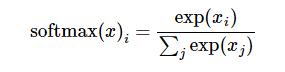,至于为什么是用的这个公式?这里不介绍了,涉及到比较多的理论证明。
第二步softmax的输出向量[Y1,Y2,Y3...]和样本的实际标签做一个交叉熵,公式如下: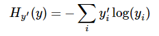
其中指代实际的标签中第i个的值(用mnist数据举例,如果是3,那么标签是`[0,0,0,1,0,0,0,0,0,0]`,除了第 4 个值为 1,其他全为 0)就是 softmax 的输出向量`[Y1, Y2, Y3...]`中,第 i 个元素的值
显而易见,预测越准确,结果的值越小(别忘了前面还有负号),最后求一个平均,得到我们想要的 loss
注意!!!这个函数的返回值并不是一个数,而是一个向量,如果要求交叉熵,我们要再做一步 tf.reduce_sum 操作,就是对向量里面所有元素求和,最后才得到,如果求 loss,则要做一步 tf.reduce_mean 操作,对向量求均值!
代码:
```python
import tensorflow as tf
#our NN's output
logits=tf.constant([[1.0,2.0,3.0],[1.0,2.0,3.0],[1.0,2.0,3.0]])
#step1:do softmax
y=tf.nn.softmax(logits)
#true label
y_=tf.constant([[0.0,0.0,1.0],[0.0,0.0,1.0],[0.0,0.0,1.0]])
#step2:do cross_entropy
cross_entropy = -tf.reduce_sum(y_*tf.log(y))
#do cross_entropy just one step
cross_entropy2=tf.reduce_sum(tf.nn.softmax_cross_entropy_with_logits(logits, y_))#dont forget tf.reduce_sum()!!
with tf.Session() as sess:
softmax=sess.run(y)
c_e = sess.run(cross_entropy)
c_e2 = sess.run(cross_entropy2)
print("step1:softmax result=")
print(softmax)
print("step2:cross_entropy result=")
print(c_e)
print("Function(softmax_cross_entropy_with_logits) result=")
print(c_e2)
```
输出结果:
```python
step1:softmax result=
[[ 0.09003057 0.24472848 0.66524094]
[ 0.09003057 0.24472848 0.66524094]
[ 0.09003057 0.24472848 0.66524094]]
step2:cross_entropy result=
1.22282
Function(softmax_cross_entropy_with_logits) result=
1.2228
```
参考:[tf.nn.softmax_cross_entropy_with_logits的用法](https://blog.csdn.net/zj360202/article/details/78582895)
关于 softmax、softmax loss、cross entropy,推荐该文,可以说讲解的非常好:**[卷积神经网络系列之softmax,softmax loss和cross entropy的讲解 - AI之路 - CSDN博客](https://blog.csdn.net/u014380165/article/details/77284921)**
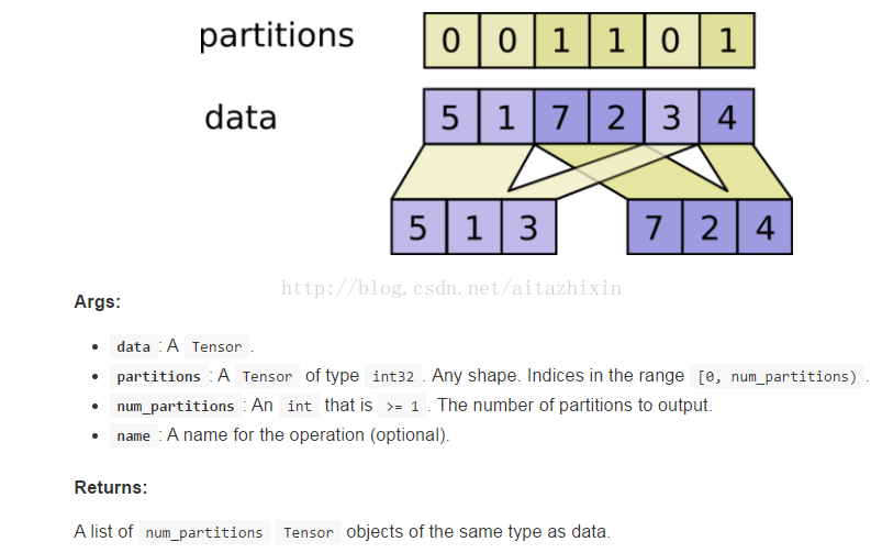
### (12) tf.dynamic_partition函数,分拆数组
拆分 Tensor:`dynamic_partition(data, partitions, num_partition, name=None)`
Tensorflow 中文社区提供的展示:
代码:
```python
# -*- coding:utf-8 -*-
import tensorflow as tf
x1 = tf.constant([[1,1],[1,1],[1,2],[1,2]], tf.float32)
x2 = tf.constant([[1,3],[1,2],[2,3],[2,4]], tf.float32)
#ones = tf.ones([2,1], dtype=tf.float32)
partitions = [1,0,1,0]
result = tf.dynamic_partition(x1, partitions, 2)
with tf.Session() as sess:
r = sess.run(result)
print r[0]
```
结果:
```python
[[ 1. 1.]
[ 1. 2.]]
```
参考:[tf.dynamic_partition 函数 分拆数组](https://blog.csdn.net/zj360202/article/details/78642340)
### (13) tf.reduce_mean等函数
tensorflow 中有一类在 tensor 的某一维度上求值的函数。如:
- 求最大值:`tf.reduce_max(input_tensor, reduction_indices=None, keep_dims=False, name=None)`
- 求平均值:`tf.reduce_mean(input_tensor, reduction_indices=None, keep_dims=False, name=None)`
参数:
- input_tensor:待求值的 tensor。
- reduction_indices:在哪一维上求解。
举例说明:
```python
# 'x' is [[1., 2.]
# [3., 4.]]
```
x 是一个 2 维数组,分别调用`reduce_*`函数如下,首先求平均值:
```python
tf.reduce_mean(x) ==> 2.5 #如果不指定第二个参数,那么就在所有的元素中取平均值
tf.reduce_mean(x, 0) ==> [2., 3.] #指定第二个参数为0,则第一维的元素取平均值,即每一列求平均值
tf.reduce_mean(x, 1) ==> [1.5, 3.5] #指定第二个参数为1,则第二维的元素取平均值,即每一行求平均值
```
指定第二个参数为 1,则第二维的元素取平均值,即每一行求平均值。
同理,还可用tf.reduce_max()求最大值等。
参考:[tensorflow官方例子中的诸如tf.reduce_mean()这类函数](https://blog.csdn.net/qq_32166627/article/details/52734387)
### (14) apply_gradients 和 compute_gradients
(1)
使用 minimize() 操作,该操作不仅可以计算出梯度,而且还可以将梯度作用在变量上。如果想在使用它们之前处理梯度,可以按照以下三步骤使用 optimizer :
```python
1. 使用函数compute_gradients()计算梯度
2. 按照自己的愿望处理梯度
3. 使用函数apply_gradients()应用处理过后的梯度
```
例如:
```python
# 创建一个optimizer.
opt = GradientDescentOptimizer(learning_rate=0.1)
# 计算相关的梯度
grads_and_vars = opt.compute_gradients(loss, )
# grads_and_vars为tuples (gradient, variable)组成的列表。
#对梯度进行想要的处理,比如cap处理
capped_grads_and_vars = [(MyCapper(gv[0]), gv[1]) for gv in grads_and_vars]
# 令optimizer运用capped的梯度(gradients)
opt.apply_gradients(capped_grads_and_vars)
```
参考:[tensorflow的模型训练Training与测试Testing等相关函数](https://blog.csdn.net/zj360202/article/details/78742523)
(2)
`apply_gradients`和`compute_gradients`是所有的优化器都有的方法。
compute_gradients:
```python
compute_gradients(
loss,
var_list=None,
gate_gradients=GATE_OP,
aggregation_method=None,
colocate_gradients_with_ops=False,
grad_loss=None
)
```
计算 loss 中可训练的 var_list 中的梯度。 相当于`minimize()`的第一步,返回 (gradient, variable) 对的 list。
apply_gradients:
```python
apply_gradients(
grads_and_vars,
global_step=None,
name=None
)
```
`minimize()`的第二部分,返回一个执行梯度更新的 ops。
例子:
```python
#Now we apply gradient clipping. For this, we need to get the gradients,
#use the `clip_by_value()` function to clip them, then apply them:
threshold = 1.0
optimizer = tf.train.GradientDescentOptimizer(learning_rate)
grads_and_vars = optimizer.compute_gradients(loss)
#list包括的是:梯度和更新变量的元组对
capped_gvs = [(tf.clip_by_value(grad, -threshold, threshold), var)
for grad, var in grads_and_vars]
#执行对应变量的更新梯度操作
training_op = optimizer.apply_gradients(capped_gvs)
```
参考:[tensorflow API:梯度修剪apply_gradients和compute_gradients](https://blog.csdn.net/NockinOnHeavensDoor/article/details/80632677)
(3)
再看一个代码:
```python
import tensorflow as tf
x = tf.Variable(tf.truncated_normal([1]), name="x")
goal = tf.pow(x-3, 2, name="goal") # y=(x-3)^2
with tf.Session() as sess:
x.initializer.run()
print(x.eval())
print(goal.eval())
optimizer = tf.train.GradientDescentOptimizer(learning_rate=0.1)
# train_step = optimizer.minimize(goal)
# 把 train_step = optimizer.minimize(goal) 拆分成计算梯度和应用梯度两个步骤。
gra_and_var = optimizer.compute_gradients(goal)
train_step = optimizer.apply_gradients(gra_and_var)
def train():
with tf.Session() as sess:
x.initializer.run()
for i in range(10):
print("x:", x.eval())
train_step.run()
print("goal:", goal.eval())
train()
```
参考:[Tensorflow 学习笔记(六)—— Optimizer](https://applenob.github.io/tf_6.html#1.-%E4%BD%BF%E7%94%A8minimize)
### (15) tf.trainable_variables和tf.all_variables的对比
tf.trainable_variables 返回的是需要训练的变量列表。
tf.all_variables 返回的是所有变量的列表。
例如:
```python
import tensorflow as tf;
import numpy as np;
import matplotlib.pyplot as plt;
v = tf.Variable(tf.constant(0.0, shape=[1], dtype=tf.float32), name='v')
v1 = tf.Variable(tf.constant(5, shape=[1], dtype=tf.float32), name='v1')
global_step = tf.Variable(tf.constant(5, shape=[1], dtype=tf.float32), name='global_step', trainable=False)
ema = tf.train.ExponentialMovingAverage(0.99, global_step)
for ele1 in tf.trainable_variables():
print ele1.name
for ele2 in tf.all_variables():
print ele2.name
```
输出:
```python
v:0
v1:0
v:0
v1:0
global_step:0
```
分析:上面得到两个变量,后面的一个得到上三个变量,因为 global_step 在声明的时候**说明不是训练变量,用来关键字 trainable=False。**
### (16) tf.control_dependencies
`tf.control_dependencies(self, control_inputs)`:
> 通过以上的解释,我们可以知道,该函数接受的参数 control_inputs,是 Operation 或者 Tensor 构成的 list。返回的是一个上下文管理器,该上下文管理器用来控制在该上下文中的操作的依赖。也就是说,上下文管理器下定义的操作是依赖 control_inputs 中的操作的,control_dependencies 用来控制 control_inputs 中操作执行后,才执行上下文管理器中定义的操作。
如果我们想要确保获取更新后的参数,name 我们可以这样组织我们的代码。
```python
opt = tf.train.Optimizer().minize(loss)
with tf.control_dependencies([opt]): #先执行opt
updated_weight = tf.identity(weight) #再执行该操作
with tf.Session() as sess:
tf.global_variables_initializer().run()
sess.run(updated_weight, feed_dict={...}) # 这样每次得到的都是更新后的weight
```
参考:[TensorFlow笔记——(1)理解tf.control_dependencies与control_flow_ops.with_dependencies](https://blog.csdn.net/liuweiyuxiang/article/details/79952493)
### (17) tf.global_variables_initializer()和tf.local_variables_initializer()区别
tf.global_variables_initializer() 添加节点用于初始化所有的变量(GraphKeys.VARIABLES)。返回一个初始化所有全局变量的操作(Op)。在你构建完整个模型并在会话中加载模型后,运行这个节点。
能够将所有的变量一步到位的初始化,非常的方便。通过 feed_dict,你也可以将指定的列表传递给它,只初始化列表中的变量。
```python
sess.run(tf.global_variables_initializer(),
feed_dict={
learning_rate_dis: learning_rate_val_dis,
adam_beta1_d_tf: adam_beta1_d,
learning_rate_proj: learning_rate_val_proj,
lambda_ratio_tf: lambda_ratio,
lambda_l2_tf: lambda_l2,
lambda_latent_tf: lambda_latent,
lambda_img_tf: lambda_img,
lambda_de_tf: lambda_de,
adam_beta1_g_tf: adam_beta1_g,
})
# learning_rate_dis为设置的变量,learning_rate_val_dis为我设置的具体的值。后续同理
```
tf.local_variables_initializer() 返回一个初始化所有局部变量的操作(Op)。初始化局部变量(GraphKeys.LOCAL_VARIABLE)。GraphKeys.LOCAL_VARIABLE 中的变量指的是被添加入图中,但是未被储存的变量。关于储存,请了解 tf.train.Saver 相关内容,在此处不详述,敬请原谅。
### (18) tf.InteractiveSession()与tf.Session()的区别
tf.InteractiveSession():它能让你在运行图的时候,插入一些计算图,这些计算图是由某些操作(operations)构成的。这对于工作在交互式环境中的人们来说非常便利,比如使用 IPython。tf.InteractiveSession() 是一种交互式的 session 方式,它**让自己成为了默认的 session**,也就是说用户在不需要指明用哪个 session 运行的情况下,就可以运行起来,这就是默认的好处。这样的话就是 run() 和 eval() 函数可以不指明 session。
tf.Session():需要在启动 session 之前构建整个计算图,然后启动该计算图。
意思就是在我们使用`tf.InteractiveSession()`来构建会话的时候,我们可以先构建一个 session 然后再定义操作(operation),如果我们使用`tf.Session()`来构建会话我们需要在会话构建之前定义好全部的操作(operation)然后再构建会话。
tf.Session()和tf.InteractiveSession()的区别他们之间的区别就是:后者加载自身作为默认的Session。tensor.eval() 和 operation.run() 可以直接使用。下面这三个是等价的:
```python
sess = tf.InteractiveSession()
```
```python
sess = tf.Session()
with sess.as_default():
```
```python
with tf.Session() as sess:
```
如下就会报错:
```python
import tensorflow as tf
a = tf.constant(4)
b = tf.constant(7)
c = a + b
sess = tf.Session()
print(c.eval())
```
如果这样就没问题:
```python
a = tf.constant(4)
b = tf.constant(7)
c = a + b
# sess = tf.Session()
with tf.Session() as sess:
print(c.eval())
```
```python
a = tf.constant(4)
b = tf.constant(7)
c = a + b
sess = tf.InteractiveSession()
print(c.eval())
```
参考:
- [TensorFlow入门:tf.InteractiveSession()与tf.Session()区别](https://blog.csdn.net/M_Z_G_Y/article/details/80416226)
- [tf.InteractiveSession()与tf.Session()](https://blog.csdn.net/qq_14839543/article/details/77822916)
- [TensorFlow(笔记):tf.Session()和tf.InteractiveSession()的区别](https://blog.csdn.net/u010513327/article/details/81023698)
### (19) tf.get_variable和tf.Variable区别
之所以会出现这两种类型的 scope,主要是后者(variable scope)为了实现 tensorflow 中的变量共享机制:即为了使得在代码的任何部分可以使用某一个已经创建的变量,TF引入了变量共享机制,使得可以轻松的共享变量,而不用传一个变量的引用。具体解释如下:
#### 1) tensorflow中创建variable的2种方式
①tf.Variable():只要使用该函数,一律创建新的variable,如果出现重名,变量名后面会自动加上后缀1,2….
```python
import tensorflow as tf
with tf.name_scope('cltdevelop):
var_1 = tf.Variable(initial_value=[0], name='var_1')
var_2 = tf.Variable(initial_value=[0], name='var_1')
var_3 = tf.Variable(initial_value=[0], name='var_1')
print(var_1.name)
print(var_2.name)
print(var_3.name)
```
结果输出如下:
```python
cltdevelop/var_1:0
cltdevelop/var_1_1:0
cltdevelop/var_1_2:0
```
②tf.get_variable():如果变量存在,则使用以前创建的变量,如果不存在,则新创建一个变量。
```python
import tensorflow as tf
with tf.name_scope("a_name_scope"):
initializer = tf.constant_initializer(value=1)
var1 = tf.get_variable(name='var1', shape=[1], dtype=tf.float32, initializer=initializer)
var2 = tf.Variable(name='var2', initial_value=[2], dtype=tf.float32)
var21 = tf.Variable(name='var2', initial_value=[2.1], dtype=tf.float32)
var22 = tf.Variable(name='var2', initial_value=[2.2], dtype=tf.float32)
with tf.Session() as sess:
sess.run(tf.initialize_all_variables())
print(var1.name) # var1:0
print(var2.name) # a_name_scope/var2:0
print(var21.name) # a_name_scope/var2_1:0
print(var22.name) # a_name_scope/var2_2:0
```
可以看出使用 tf.Variable() 定义的时候, 虽然 name 都一样, 但是为了不重复变量名, Tensorflow 输出的变量名并不是一样的. 所以, 本质上 var2, var21, var22 并不是一样的变量. 而另一方面, 使用 tf.get_variable() 定义的变量不会被 tf.name_scope() 当中的名字所影响.
如果想要达到重复利用变量的效果, 我们就要使用 tf.variable_scope(),并搭配 tf.get_variable() 这种方式产生和提取变量. 不像 tf.Variable() 每次都会产生新的变量,tf.get_variable() **如果遇到了同样名字的变量时, 它会单纯的提取这个同样名字的变量(避免产生新变量)。** 而在重复使用的时候, 一定要在代码中强调 scope.reuse_variables(),否则系统将会报错,以为你只是单纯的不小心重复使用到了一个变量。来源:[TensorFlow之scope命名方式](https://blog.csdn.net/buddhistmonk/article/details/79769828)
#### 2) tensorflow中的两种作用域
1. 命名域(name scope):通过 tf.name_scope() 来实现;
变量域(variable scope):通过 tf.variable_scope() 来实现;可以通过设置 reuse 标志以及初始化方式来影响域下的变量。
2. 这两种作用域都会给 tf.Variable() 创建的变量加上词头,而 tf.name_scope 对 tf.get_variable() 创建的变量没有词头影响,代码如下:
```python
import tensorflow as tf
with tf.name_scope('cltdevelop'):
var_1 = tf.Variable(initial_value=[0], name='var_1')
var_2 = tf.get_variable(name='var_2', shape=[1, ])
with tf.variable_scope('aaa'):
var_3 = tf.Variable(initial_value=[0], name='var_3')
var_4 = tf.get_variable(name='var_4', shape=[1, ])
print(var_1.name)
print(var_2.name)
print(var_3.name)
print(var_4.name)
```
结果输出如下:
```python
cltdevelop/var_1:0
var_2:0
aaa/var_3:0
aaa/var_4:0
```
#### 3) tensorflow中变量共享机制的实现
在 tensorflow 中变量共享机制是通过 tf.get_variable() 和 tf.variable_scope() 两者搭配使用来实现的。如下代码所示:
```python
import tensorflow as tf
with tf.variable_scope('cltdevelop'):
var_1 = tf.get_variable('var_1', shape=[1, ])
with tf.variable_scope('cltdevelop', reuse=True):
var_2 = tf.get_variable('var_1', shape=[1,])
print(var_1.name)
print(var_2.name)
```
结果输出如下:
```python
cltdevelop/var_1:0
cltdevelop/var_1:0
```
注:当 reuse 设置为 True 或者 tf.AUTO_REUSE 时,表示这个 scope 下的变量是重用的或者共享的,也说明这个变量以前就已经创建好了。但如果这个变量以前没有被创建过,则在 tf.variable_scope 下调用 tf.get_variable 创建这个变量会报错。如下:
```python
import tensorflow as tf
with tf.variable_scope('cltdevelop', reuse=True):
var_1 = tf.get_variable('var_1', shape=[1, ])
```
则上述代码会报错:
```python
ValueErrorL Variable cltdevelop/v1 doesnot exist, or was not created with tf.get_variable()
```
### (20) tf.where()用法
`where(condition, x=None, y=None, name=None)`的用法:
condition, x, y 相同维度,condition 是 bool 型值,True/False。
返回值是对应元素,condition 中元素为 True 的元素替换为 x 中的元素,为 False 的元素替换为 y 中对应元素,x 只负责对应替换 True 的元素,y 只负责对应替换 False 的元素,x,y 各有分工,由于是替换,返回值的维度,和condition,x , y 都是相等的。
看个例子:
```python
import tensorflow as tf
x = [[1,2,3],[4,5,6]]
y = [[7,8,9],[10,11,12]]
condition3 = [[True,False,False],
[False,True,True]]
condition4 = [[True,False,False],
[True,True,False]]
with tf.Session() as sess:
print(sess.run(tf.where(condition3,x,y)))
print(sess.run(tf.where(condition4,x,y)))
```
参考:[tenflow 入门 tf.where()用法](https://blog.csdn.net/ustbbsy/article/details/79564828)
### (21) tf.less()用法
`less(x, y, name=None)`:以元素方式返回(x 从输出可以看到,均匀分布生成的随机数并不是从小到大或者从大到小均匀分布的,这里均匀分布的意义是每次从一组服从均匀分布的数里边随机抽取一个数。
>
> tf中另一个生成均匀分布的类是 tf.uniform_unit_scaling_initializer(),同样都是生成均匀分布,tf.uniform_unit_scaling_initializer 跟 tf.random_uniform_initializer 不同的地方是前者不需要指定最大最小值,是通过公式计算出来的:
>
> ```python
> max_val = math.sqrt(3 / input_size) * factor
> min_val = -max_val
> ```
- 初始化为变尺度正太、均匀分布,tf 中 tf.variance_scaling_initializer() 类可以生成截断正太分布和均匀分布的 tensor,增加了更多的控制参数。
- 其他初始化方式
- tf.orthogonal_initializer() 初始化为正交矩阵的随机数,形状最少需要是二维的
- tf.glorot_uniform_initializer() 初始化为与输入输出节点数相关的均匀分布随机数
- tf.glorot_normal_initializer() 初始化为与输入输出节点数相关的截断正太分布随机数
#### tf.truncated_normal的用法
#### tf.truncated_normal(shape, mean, stddev)
shape 表示生成张量的维度,mean 是均值,stddev 是标准差。这个函数产生正太分布,均值和标准差自己设定。这是一个截断的产生正太分布的函数,就是说产生正太分布的值如果与均值的差值大于两倍的标准差,那就重新生成。和一般的正太分布的产生随机数据比起来,这个函数产生的随机数与均值的差距不会超过两倍的标准差,但是一般的别的函数是可能的。注:关于什么是标准差推荐阅读该文【[标准差和方差](https://www.shuxuele.com/data/standard-deviation.html)】。
代码:
```python
import tensorflow as tf;
import numpy as np;
import matplotlib.pyplot as plt;
c = tf.truncated_normal(shape=[10,10], mean=0, stddev=1)
with tf.Session() as sess:
print sess.run(c)
```
参考:[tf.truncated_normal的用法](https://blog.csdn.net/UESTC_C2_403/article/details/72235565)
### (24) 优化器
Tensorflow 提供了下面这些种优化器:
- tf.train.GradientDescentOptimizer
- tf.train.AdadeltaOptimizer
- tf.train.AdagradOptimizer
- tf.train.AdagradDAOptimizer
- tf.train.MomentumOptimizer
- tf.train.AdamOptimizer
> AdamOptimizer 通过使用动量(参数的移动平均数)来改善传统梯度下降,促进超参数动态调整。
>
> 自适应优化算法通常都会得到比SGD算法性能更差(经常是差很多)的结果,尽管自适应优化算法在训练时会表现的比较好,因此使用者在使用自适应优化算法时需要慎重考虑!(终于知道为啥CVPR的paper全都用的SGD了,而不是用理论上最diao的Adam)。来源:[随机最速下降法(SGD)与AdamOptimizer](https://blog.csdn.net/weixin_38145317/article/details/79346242)
- tf.train.FtrlOptimizer
- tf.train.ProximalGradientDescentOptimizer
- tf.train.ProximalAdagradOptimizer
- tf.train.RMSPropOptimizer
各种优化器对比:
- 标准梯度下降法:标准梯度下降先计算所有样本汇总误差,然后根据总误差来更新权值
- 随机梯度下降法:随机梯度下降随机抽取一个样本来计算误差,然后更新权值
- 批量梯度下降法:批量梯度下降算是一种折中的方案,从总样本中选取一个批次(比如一共有 10000 个样本,随机选取 100 个样本作为一个 batch),然后计算这个 batch 的总误差,根据总误差来更新权值。
> 标准梯度下降法:先计算所有样本汇总误差,然后根据总误差来更新全值(时间长,值更加可靠)
> 随机梯度下降法:随机抽取一个样本来计算误差,然后更新权值(时间短,值相对不可靠)
> 批量梯度下降法:从总样本中选取一个批次,然后计算这个batch的总误差,根据总误差来更新权值(折中)
>
> *来源:知乎 [知乎ID-鹏](https://www.zhihu.com/question/63235995/answer/452385142)*
更多内容:
- [TensorFlow学习(四):优化器Optimizer](https://blog.csdn.net/xierhacker/article/details/53174558)
- [AI学习笔记——Tensorflow中的Optimizer(优化器)](https://www.afenxi.com/59457.html)
- [TensorFlow 学习摘要(三) 深度学习 - TensorFlow 优化器](http://blog.720ui.com/2018/tensorflow_03_dl_tensorflow_optimizer/)
### (25) 损失函数(或代价函数)
在机器学习中,loss function(损失函数)也称 cost function(代价函数),是用来计算预测值和真实值的差距。 然后以 loss function 的最小值作为目标函数进行反向传播迭代计算模型中的参数,这个让 loss function 的值不断变小的过程称为优化。
常见的损失函数:`Zero-one Loss`(0-1损失),`Perceptron Loss`(感知损失),`Hinge Loss`(Hinge损失),`Log Loss`(Log损失),`Cross Entropy`(交叉熵),`Square Loss`(平方误差)`,`Absolute Loss`(绝对误差)`,`Exponential Loss`(指数误差)等
一般来说,对于分类或者回归模型进行评估时,需要使得模型在训练数据上的损失函数值最小,即使得经验风险函数(Empirical risk)最小化,但是如果只考虑经验风险,容易出现过拟合,因此还需要考虑模型的泛化性,一般常用的方法就是在目标函数中加上正则项,由**损失项(loss term)加上正则项(regularization term)构成结构风险(Structural risk)**,那么损失函数变为: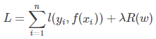
其中 λ 为正则项超参数,常用的正则化方法包括:**L1正则和L2正则**。
#### tf.nn.softmax_cross_entropy_with_logits
用法见:【[(11) tf.nn.softmax_cross_entropy_with_logits的用法](#11-tfnnsoftmax_cross_entropy_with_logits的用法)】
#### tf.nn.sparse_softmax_cross_entropy_with_logits(logits, labels, name=None)
该函数与 tf.nn.softmax_cross_entropy_with_logits() 函数十分相似,**唯一的区别在于 labels 的 shape,该函数的labels要求是排他性的即只有一个正确的类别,** 如果 labels 的每一行不需要进行 one_hot 表示,可以使用 tf.nn.sparse_softmax_cross_entropy_with_logits( )。
> (1)
>
> 这个函数和 tf.nn.softmax_cross_entropy_with_logits 函数比较明显的区别在于它的参数 labels 的不同,这里的参数 label 是非稀疏表示的,比如表示一个 3 分类的一个样本的标签,稀疏表示的形式为 [0, 0, 1] 这个表示这个样本为第 3 个分类,而非稀疏表示就表示为 2(因为从 0 开始算,0,1,2, 就能表示三类),同理[0,1,0]就表示样本属于第二个分类,而其非稀疏表示为 1。tf.nn.sparse_softmax_cross_entropy_with_logits() 比 tf.nn.softmax_cross_entropy_with_logits 多了一步将 labels 稀疏化的操作。因为深度学习中,图片一般是用非稀疏的标签的,所以用 tf.nn.sparse_softmax_cross_entropy_with_logits() 的频率比 tf.nn.softmax_cross_entropy_with_logits 高。*——form:[tf.nn.sparse_softmax_cross_entropy_with_logits()](https://blog.csdn.net/m0_37041325/article/details/77043598)*
>
> (2)
>
> 相同点:tf.nn.sparse_softmax_cross_entropy_with_logits() 与 tf.nn.softmax_cross_entropy_with_logits() 这两个函数都是对输出的预测结果(logits)进行 softmax 操作然后再计算与真实值(labels)的交叉熵。
>
> 不同点:输入有一处不同,tf.nn.sparse_softmax_cross_entropy_with_logits() 的真实值(labels)要求是一个数,而 tf.nn.softmax_cross_entropy_with_logits() 的真实值(labels)要求是一个列表。
>
> 例如,对于手写字体分类问题,并假设这张图片所代表的的数字是 8,那么在使用 tf.nn.sparse_softmax_cross_entropy_with_logits() 时,labels 参数要赋值为 8,而若使用 tf.nn.softmax_cross_entropy_with_logits(),labels 参数要赋值为 [0, 0, 0, 0, 0, 0, 0, 0, 1, 0]。如果要使用 tf.nn.sparse_softmax_cross_entropy_with_logits(),但数据集给的是 [0, 0, 0, 0, 0, 0, 0, 0, 1, 0] 这种形式,那么可以使用 tf.argmax() 这个函数来取得 8 这个值。*——from:*
>
> (3)
>
> 如果看 tensorflow 源码,比较容易能看出来这两者的区别。以基本的 mnist 分类场景有例,mnist 有 10 类,训练时的 batch size 为 batch_num
>
> 1. 则若使用 softmax_cross_entropy_with_logits, 则其 labels 参数需要是一个`[batch_size, 10]`的矩阵,其中每行代表一个 instance, 是 one hot 的形式,其非0 index代表属于哪一类。
> 2. 若使用 sparse_softmax_cross_entropy_with_logits, 则其 labels 参数是一个`[batch_size]`的列,里面每个属于 0 到 9 中间的整数,代表类别,所以函数名称加了 sparse,类似稀疏表示。
>
> *——from:*
#### tf.nn.sigmoid_cross_entropy_with_logits(logits, targets, name=None)
sigmoid_cross_entropy_with_logits 是 TensorFlow 最早实现的交叉熵算法。这个函数的输入是 logits 和 labels,logits 就是神经网络模型中的 `W*X` 矩阵,注意不需要经过 sigmoid ,而 labels 的 shape 和 logits 相同,就是正确的标签值,例如这个模型一次要判断 100 张图是否包含 10 种动物,这两个输入的 shape 都是 [100, 10]。**注释中还提到这10个分类之间是独立的、不要求是互斥,这种问题我们称为多目标(多标签)分类,例如判断图片中是否包含10种动物中的一种或几种,标签值可以包含多个 1 或 0 个 1**。
#### tf.nn.weighted_cross_entropy_with_logits(logits, targets, pos_weight, name=None)
weighted_sigmoid_cross_entropy_with_logits 是 sigmoid_cross_entropy_with_logits 的拓展版,多支持一个 pos_weight 参数,在传统基于 sigmoid 的交叉熵算法上,正样本算出的值乘以某个系数。
### (26) 设置自动衰减的学习率
在训练神经网络的过程中,合理的设置学习率是一个非常重要的事情。对于训练一开始的时候,设置一个大的学习率,可以快速进行迭代,在训练后期,设置小的学习率有利于模型收敛和稳定性。
```python
tf.train.exponential_decay(learing_rate, global_step, decay_steps, decay_rate, staircase=False)
```
- learning_rate:学习率
- global_step:全局的迭代次数
- decay_steps:进行一次衰减的步数
- decay_rate:衰减率
- staircase:默认为 False,如果设置为 True,在修改学习率的时候会进行取整
转换方程:
实例:
```python
import tensorflow as tf
import matplotlib.pyplot as plt
start_learning_rate = 0.1
decay_rate = 0.96
decay_step = 100
global_steps = 3000
_GLOBAL = tf.Variable(tf.constant(0))
S = tf.train.exponential_decay(start_learning_rate, _GLOBAL, decay_step, decay_rate, staircase=True)
NS = tf.train.exponential_decay(start_learning_rate, _GLOBAL, decay_step, decay_rate, staircase=False)
S_learning_rate = []
NS_learning_rate = []
with tf.Session() as sess:
for i in range(global_steps):
print(i, ' is training...')
S_learning_rate.append(sess.run(S, feed_dict={_GLOBAL: i}))
NS_learning_rate.append(sess.run(NS, feed_dict={_GLOBAL: i}))
plt.figure(1)
l1, = plt.plot(range(global_steps), S_learning_rate, 'r-')
l2, = plt.plot(range(global_steps), NS_learning_rate, 'b-')
plt.legend(handles=[l1, l2, ], labels=['staircase', 'no-staircase'], loc='best')
plt.show()
```
该实例表示训练过程总共迭代 3000 次,每经过 100 次,就会对学习率衰减为原来的 0.96。
参考:
- [设置自动衰减的学习率](https://blog.csdn.net/TwT520Ly/article/details/80402803)
- [Tensorflow实现学习率衰减](https://blog.csdn.net/u013555719/article/details/79334359)
### (27) 命令行参数
第一种:利用 python 的 argparse 包
第二种:tensorflow 自带的 app.flags 实现
参考:[[干货|实践] Tensorflow学习 - 使用flags定义命令行参数](https://zhuanlan.zhihu.com/p/33249875)