VASP光学性质计算
注:本文档为个人经验之谈,已经尽可能减少歧义,不保证完全正确!本文档后半部分译自VASPKIT官方手册,如有不当之处请读者查阅原文。
1. 结构优化
为了进行 VASP计算,通常需要4个文件:INCAR、POSCAR、POTCAR和 KPOINTS。
INCAR包含所有关键词,告诉VASP需要计算什么;POSCAR包含晶格参数、原子坐标信息和原子速度信息(用于分子动力学);POTCAR是一个赝势文件,类型可以是超软赝势(USPP)或者投影缀加波(PAW);KPOINTS文件,虽然可以包含在INCAR中,但不建议省略。它包含倒易空间中的K点信息,波函数在这些点上进行积分以获得电荷密度。
解释补充:
INCAR是控制计算的主要输入文件POSCAR定义了体系的结构信息POTCAR描述了电子-离子相互作用KPOINTS对计算精度和效率都很重要
这四个文件是 VASP计算的基本输入文件,缺一不可。
建立
opt文件夹,在包含POSCAR(优先执行第三步)的目录中运行VASPKIT。输入1选择函数VASP Input Files Generator,然后输入101选择自定义INCAR文件:
SYSTEM=tio2au #此处命名随意
ISTART =  0            (Read existing wavefunction; if there)
ISPIN  =  1            (Non-Spin polarised DFT)
# ICHARG =  11         (Non-self-consistent: GGA/LDA band structures)
LREAL  = Auto          (Projection operators: automatic)
ENCUT  =  500        (Cut-off energy for plane wave basis set, in eV)
PREC   =  Accurate       (Precision level)
LWAVE  = .F.        (Write WAVECAR or not)
LCHARG = .F.        (Write CHGCAR or not)
ADDGRID= .TRUE.        (Increase grid; helps GGA convergence)
NPAR   = 4           (Max is no. nodes; don't set for hybrids)
Nwrite = 2           (Medium-level output)

#Electronic Relaxation
ISMEAR =  0            (Gaussian smearing; metals:1)
SIGMA  =  0.05         (Smearing value in eV; metals:0.2)
NELM   =  200           (Max electronic SCF steps)
NELMIN =  6            (Min electronic SCF steps)
EDIFF  =  1E-08        (SCF energy convergence; in eV)

#Ionic Relaxation
NSW    =  200          (Max ionic steps)
IBRION =  2            (Algorithm: 0-MD; 1-Quasi-New; 2-CG)
ISIF   =  2            (Stress/relaxation: 2-Ions, 3-Shape/Ions/V, 4-Shape/Ions)
EDIFFG = -2E-02        (Ionic convergence; eV/AA)

#DFT+U Calculation for Ti atoms
LDAU   = .TRUE.        (Activate DFT+U)
LDATYPE=  2            (Dudarev; only U-J matters)
LDAUL  =  -1 2 -1         (Orbitals for each species)
LDAUU  =  0 6.0 0         (U for each species)
LDAUJ  =  0 0.5 0         (J for each species)
LMAXMIX=  4            (Mixing cut-off; 4-d, 6-f)

#DFT-D3 Correction
IVDW   =  12           (DFT-D3BJ method of method with no damping)
使用
vaspkit工具(下载地址)生成KPOINTS文件(功能102): 输入1以选择原始 Monkhorst-Pack 方案,输入2以选择 Gamma 为中心的 Monkhorst-Pack 方案。
K-Spacing Value to Generate K-Mesh: 0.040
0
Monkhorst-Pack
    3   7   1
0.0    0.0  0.0
利用
M$生成晶胞(或者其他软件如ASE),然后使用xsd2pos_v2.1.pl脚本生成POSCAR文件(或自己手动书写)。源码:复制下面代码并命名为xsd2pos_v2.1.pl文件。VASPKIT 可以通过选项
105和106将 .cif 和 .xsd(Materials Studio 格式)文件转换为 POSCAR 格式。105将调用/vaspkit.1.00/utilities/cif2pos.py脚本。106将自动调用/vaspkit.1.00/utilities/xsd2pos.py脚本。请注意,.xsd 文件中的 Atom 修复信息在 transform 时保留。107可以对 POSCAR 文件中的元素进行重新排序。
#!perl
#This is perl script for converting the Materials Studio xsd file to the POSCAR file for VASP.
#xsd2pos.pl can read the constraints information from the xsd file, and write the constraints to the POSCAR file.
#Usage: Change the $filename variable to your xsd file, and it will generate a POSCAR.txt file in the VASP input format. You may copy and paste the text in POSCAR.txt to your POSCAR file.

use strict;
use Getopt::Long;
use MaterialsScript qw(:all);

my $filename = "type_the_filename_here";
my $doc = $Documents{"$filename.xsd"};
my $pos = Documents->New("POSCAR.txt");
my $lattice = $doc->SymmetryDefinition;
my $FT;
my @num_atom;
my @element;
my $ele;
my $num;
my $testif;
my $FT1;
my $FT2;
my $FT3;

$pos->Append(sprintf "$filename \n");
$pos->Append(sprintf "1.0 \n");
$pos->Append(sprintf "%f %f %f \n",$lattice->VectorA->X, $lattice->VectorA->Y, $lattice->VectorA->Z);
$pos->Append(sprintf "%f %f %f \n",$lattice->VectorB->X, $lattice->VectorB->Y, $lattice->VectorB->Z);
$pos->Append(sprintf "%f %f %f \n",$lattice->VectorC->X, $lattice->VectorC->Y, $lattice->VectorC->Z);


my $atoms = $doc->UnitCell->Atoms;

my @sortedAt = sort {$a->AtomicNumber <=> $b->AtomicNumber} @$atoms;

my $count_el=0;
my $count_atom = 0;
   $element[0]=$sortedAt[0]->ElementSymbol;
my $atom_num = $sortedAt[0]->AtomicNumber;
foreach my $atom (@sortedAt) {
  if ($atom->AtomicNumber == $atom_num) {
    $count_atom=$count_atom+1;
  } else {
    $num_atom[$count_el] = $count_atom;
    $count_atom = 1;
    $count_el = $count_el+1;
    $element[$count_el]=$atom->ElementSymbol;
    $atom_num = $atom->AtomicNumber;
  }
}
$num_atom[$count_el] = $count_atom;

foreach $ele (@element) {
   $pos->Append(sprintf "$ele ");
}
$pos->Append(sprintf "\n");

foreach $num (@num_atom) {
   $pos->Append(sprintf "$num ");
}
$pos->Append(sprintf "\n");
$pos->Append(sprintf "Selective Dynamics\nDirect \n");

foreach my $atom (@sortedAt) {

 if ($atom->IsFixed("X")) {
    $FT1 = "F";
 } else {
    $FT1 = "T";
 }
 if ($atom->IsFixed("Y")) {
    $FT2 = "F";
 } else {
    $FT2 = "T";
 }
 if ($atom->IsFixed("Z")) {
    $FT3 = "F";
 } else {
    $FT3 = "T";
 }

if ($atom->IsFixed("FractionalXYZ")) {
    $FT = "F F F";
 } elsif ($atom->IsFixed("XYZ")) {
    $FT = "F F F";
} else {
    $FT = "$FT1 $FT2 $FT3";
}

$pos->Append(sprintf "%f %f %f %s \n", $atom->FractionalXYZ->X, $atom->FractionalXYZ->Y, $atom->FractionalXYZ->Z, $FT);
# $pos->Append(sprintf "%s %d %f %f %f %s \n", $atom->ElementSymbol, $atom->AtomicNumber, $atom->FractionalXYZ->X, $atom->FractionalXYZ->Y, $atom->FractionalXYZ->Z, $FT);
}
生成
POTCAR文件:此处需要VASP的赝势库。然后在vaspkit的设置文件中(~/.vaspkit)定义赝势库的位置。然后在vaspkit中使用103功能生成POTCAR文件。此外,也可以手动导入赝势库中的原子信息,例:GeS
cat ~/xxx/PBE/Ge/POTCAR > POTCAR # ~/xxx 为赝势库存放路径
cat ~/xxx/PBE/S/POTCAR >> POTCAR # 原子赝势导入顺序以POSCAR中为准
注:在生成
KPOINTS时,POTCAR也会自动生成。或者运行VASPKIT103生成POTCAR。它从POSCAR中读取元素信息,并组合您在~/.vaspkit中设置的赝势文件夹中的相应POTCAR。根据需要将POTCAR_TYPE设置为PBE、GGA或LDA。RECOMMENDED_POTCAR标签控制是否使用 VASP 手册(第 195 页,2018.10.29,http://cms.mpi.univie.ac.at/vasp/vasp/Recommended_PAW_potentials_DFT_calculations_using_vasp_5_2.html 页)中的推荐势。如果RECOMMENDED_POTCAR为.FALSE.,则将使用不带扩展名的 POTCAR。如果RECOMMENDED_POTCAR为.TRUE.,官方推荐的 POTCAR 将被使用。POTCAR 类型:
无扩展名 “_”
_d扩展 d,将 d 半核心状态视为价态。_pv或_sv。扩展_pv和_sv意味着p 和 s 半核态被视为价态。_h和_s。扩展_h_s意味着电位比标准电位更硬或更软,因此需要更高或更低的能量截止。赝氢。例如:
H.5_GW。用于 GW 计算。
如果要生成 POTCAR 进行 GW 计算,请将
GW_POTCAR设置为.TRUE.在~/.vaspkit中。VASPKIT 还提供
104个选项,通过为每个元素选择势类型来手动生成 POTCAR。
VASPKIT 可以通过选项
109进行格式校正和伪电位检查。VASPKIT 将自动更正 INCAR 和 POSCAR 格式,并检查 POTCAR 和 POSCAR 是否一致。如果是集群,还需要提交作业的脚本,以
slurm系统为例:
#!/bin/bash
#SBATCH -J vasp_tio2au
#SBATCH -o %J.out
#SBATCH -e %J.err
#SBATCH -N 1
#SBATCH -w node01
#SBATCH -n 64
#SBATCH -t 30-12:00:00
#SBATCH -p hpc
###SBATCH --dependency=afterok:0
#=======================
export OMP_NUM_THREADS=1
export I_MPI_ADJUST_REDUCE=3
#=======================
echo =======================
echo Submit Time is [`date`].
echo Working dir is [$SLURM_SUBMIT_DIR].
cd $SLURM_SUBMIT_DIR
NPROCS=$((SLURM_NTASKS))
N_NODE=$((SLURM_JOB_NUM_NODES))
echo This job has allocated [${N_NODE}] nodes with [${NPROCS}] processors.
echo Running on host [`hostname`].
echo This jobs runs on the following processors:
echo =======================
echo "**Start!!!"
echo Job start Time is [`date`].
echo This job name is [$SLURM_JOB_NAME] and job id is [$SLURM_JOB_ID]. >> $SLURM_JOB_ID.out
echo =======================
#=======================
source ~/.bashrc
source /data1/soft_bashrc/before_run_vasp_and_tools.sh
export GPAW_SETUP_PATH=gpaw-setups

start_time=$(date +%s)

# 1
task_start_time=$(date +%s)
mpirun -np $NPROCS vasp_std >& screen.log
task_duration=$(( $(date +%s) - $task_start_time ))
echo "Task 1 duration: $task_duration seconds." >> $SLURM_JOB_ID.out

end_time=$(date +%s)
duration=$(( $end_time - $start_time ))
echo "Total duration: $duration seconds." >> $SLURM_JOB_ID.out

echo Job finish Time is [`date`].
echo "**Finished!!!"
echo =======================
echo "                       "
提交作业:
sbatch job.sh计算结束后,
cat OUTCAR查看体系是否收敛,如收敛则进入下一步计算。
2. 静态自洽
建立
scf文件夹,编辑以下文件
1. INCAR
SYSTEM=tio2au_vacancy
ISTART =  0            (Read existing wavefunction; if there)
ISPIN  =  1            (Non-Spin polarised DFT)
# ICHARG =  11         (Non-self-consistent: GGA/LDA band structures)
LREAL  = Auto          (Projection operators: automatic)
ENCUT  =  500        (Cut-off energy for plane wave basis set, in eV)
PREC   =  Accurate       (Precision level)
#LWAVE  = .F.        (Write WAVECAR or not) #修改
#LCHARG = .F.        (Write CHGCAR or not)  #修改
ADDGRID= .TRUE.        (Increase grid; helps GGA convergence)
NPAR   = 4           (Max is no. nodes; don't set for hybrids)
Nwrite = 2           (Medium-level output)

#Electronic Relaxation
ISMEAR =  0            (Gaussian smearing; metals:1)
SIGMA  =  0.05         (Smearing value in eV; metals:0.2)
NELM   =  200           (Max electronic SCF steps)
NELMIN =  6            (Min electronic SCF steps)
EDIFF  =  1E-08        (SCF energy convergence; in eV)

#Ionic Relaxation
NSW    =  0          (Max ionic steps)   #修改
IBRION =  2            (Algorithm: 0-MD; 1-Quasi-New; 2-CG)
ISIF   =  2            (Stress/relaxation: 2-Ions, 3-Shape/Ions/V, 4-Shape/Ions)
EDIFFG = -2E-02        (Ionic convergence; eV/AA)

#DFT+U Calculation for Ti atoms
LDAU   = .TRUE.        (Activate DFT+U)
LDATYPE=  2            (Dudarev; only U-J matters)
LDAUL  =  -1 2 -1         (Orbitals for each species)
LDAUU  =  0 6.0 0         (U for each species)
LDAUJ  =  0 0.5 0         (J for each species)
LMAXMIX=  4            (Mixing cut-off; 4-d, 6-f)

#DFT-D3 Correction
IVDW   =  12           (DFT-D3BJ method of method with no damping)
2. KPOINTS
K-Spacing Value to Generate K-Mesh: 0.040
0
Monkhorst-Pack
   6   14   1 # 较opt选取,K值增大
0.0  0.0  0.0
3. POSCAR和 POTCAR
cp ../opt/CONTCAR POSCAR
cp ../opt/POTCAR .
提交作业,产生
WAVECAR文件进行下一步计算(记得检查一下计算是否正常结束)
3. 能带结构
要进行能带结构计算,需要准备一个原始单元和对应的 K 点路径 (K-path) 单独 Irreducible BrillouinZone。不可约布里渊区是由晶格的点群(晶体的点群)中的所有对称性简化的第一个布里渊区。识别并选择高对称点,并将它们沿不可简化布里渊区的边缘连接起来。
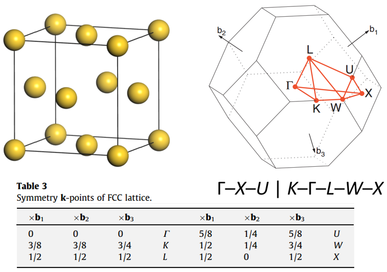
例如,常规 FCC 金属电池、不可约布里渊区和高对称点:
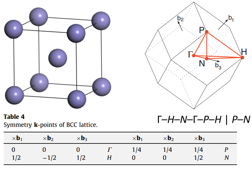
传统的 BCC 金属细胞、不可还原的布里渊区和高对称点:
K-path 并非唯一。通常,没有必要选择所有高对称点之间的所有线。在 KPOINTS 文件中选择具有代表性和重要性的线并写入线模式。对于大规模和高吞吐量计算,应该有一个规则来定义结构信息的路径。pymatgen 和 seeK-path 提供了一些解决方案,但只能用于 3D 系统。VASPKIT 提供了一种工具,用于根据系统规则为 1D(任务
301)、2D(任务302)和 3D(任务303)材料生成 K 路径:使用 pymatgen(https://pymatgen.org/)计算材料科学 49(2010) 299–312.seek-path(https://www.materialscloud.org/work/tools/seekpath)计算材料科学 128 (2017) 140–184.
对于建议的散装材料 k 路径,VASPKIT 使用与 seek-path 网站相同的算法(Y. Hinuma、G. Pizzi、Y. Kumagai、F. Oba、I. Tanaka、基于晶体学的带结构图路径,Comp. Mat. Sci. 128, 140 (2017)。
示例:单层 MoS2
1. 准备能用于能带计算的POSCAR文件(素晶胞)
因为 VASPKIT 生成的 K-path 是基于标准化原胞的,所以请先标准化 POSCAR。对于 2D 材质:将 2D 材质的 z 坐标中心保持在 | c |/2.(即分数坐标 z = 0.5 )。这可以通过 VASPKIT
921或923来完成。VASPKIT923标准化了 2D 晶体单元,(i) 将真空层置于 z 方向,(ii) 将 2D 材料置于 z 坐标的中心:对于 3D 材质,请使用 VASPKIT
602生成标准化原胞PRIMCELL.vasp,并替换原始 POSCAR。(原胞——素晶胞)以下是 MoS2 的标准化 POSCAR:
MoS2
1.0
        3.1659998894         0.0000000000         0.0000000000
        -1.5829999447         2.7418363326         0.0000000000
        0.0000000000         0.0000000000        18.4099998474
      S   Mo
      2    1
Direct
      0.000000000         0.000000000         0.413899988
      0.000000000         0.000000000         0.586099982
      0.666666687         0.333333343         0.500000000
92
+-------------------------- Warm Tips --------------------------+
            Please Use These Features with CAUTION!
+---------------------------------------------------------------+
===================== 2D Materials Toolkit ======================
921) Center Aomic-Layer along z direction
922) Resize Vacuum Thickness
923) Standardize 2D Crystal Cell
926) Elastic Constants for 2D Materials
927) Valence and Conduction Band Edges Referenced to Vacuum Level
929) Summary for Relaxed 2D Structure

0)   Quit
9)   Back
------------>>
923
-->> (1) Reading Structural Parameters from POSCAR File...
-->> (2) Written POSCAR_NEW File!
进行几何优化,然后进行单点自洽计算(计算方法保持一致),得到 CHGCAR(能带计算时要读取该文件)。
然后将计算素晶胞的scf数据复制一份用于能带计算:
cp -rf scf band
2. 准备KPOINTS文件(K路径)
在新文件夹中运行 VASPKIT
302,获取 2D K-path 文件:(注意:请检查 Space Group)302 +-------------------------- Warm Tips --------------------------+ See An Example in vaspkit/examples/seek_kpath/graphene_2D. This feature is still experimental & check the PRIMCELL.vasp file. +---------------------------------------------------------------+ -->> (1) Reading Structural Parameters from POSCAR File... +-------------------------- Summary ----------------------------+ The vacuum slab is supposed to be along c axis Prototype: AB2 Total Atoms in Input Cell: 3 Lattice Constants in Input Cell: 3.166 3.166 18.410 Lattice Angles in Input Cell: 90.000 90.000 120.000 Total Atoms in Primitive Cell: 3 Lattice Constants in Primitive Cell: 3.166 3.166 18.410 Lattice Angles in Primitive Cell: 90.000 90.000 120.000 2D Bravais Lattice: Hexagonal Space Group: 187 Point Group: 26 [ D3h ] International: P-6m2 Symmetry Operations: 12 Suggested K-Path: (shown in the next line) [ GAMMA-M-K-GAMMA ] +---------------------------------------------------------------+ -->> (2) Written PRIMCELL.vasp file. -->> (3) Written KPATH.in File for Band-Structure Calculation. -->> (4) Written HIGH_SYMMETRY_POINTS File for Reference.
KPATH.in文件包含线模式K-path。复制到 KPOINTScp KPATH.in KPOINTS。默认交叉点为 20。HIGH_SYMMETRY_POINTS 包括所有高对称点的信息。VASPKIT 不保证 K-path 是正确的,请比较 seeK-pathwebsite(https://www.materialscloud.org/work/tools/seekpath) 的结果。或者使用
303功能生成3DK-Path。然后复制为KPOINTS。
3. 准备INCAR文件
   ##### initial I/O #####
   SYSTEM = MoS2
   ISTART=1 # 修改
   ICHARG = 11 # 从CHGCAR中读入电荷分布,并且在计算中保持不变
   LWAVE = .TRUE.  # 修改 读取
   LCHARG = .TRUE.  # 修改
   LVTOT = .FALSE.
   LVHAR = .FALSE.
   LELF = .FALSE.
   LORBIT = 11 # 增加
   NEDOS = 1000 # 增加

   ##### SCF #####
   ENCUT = 500
   ISMEAR = 0
   SIGMA = 0.05
   EDIFF = 1E-6
   NELMIN = 5
   NELM = 300
   GGA = PE
   LREAL = .FALSE.
   PREC = Accurate # 保证该参数和scf计算时一致
4. 从单点计算中读取 CHGCAR 并提交 VASP 能带结构作业。
5. 一些技巧:
   alias gk="~/software/ktool/gk.x"
   alias pb="~/software/ktool/pbnf.x"
   alias f="grep E-fermi OUTCAR"
   alias lv="grep -A3 'lattice vectors' OUTCAR"
   # 实坐标与虚坐标通过命令lv得到,费米能级通过命令f得到
   # 输入命令gk获取KOINTS文件,若文件后有多行零,则删去,且第二行数据减去相应删去行数。
   提交作业,计算结束后生成 EIGENVAL 文件,输入命令pb得到能带数据文件 bnd.dat 和 highk.dat,将数据导入Origin绘图。
6. 后处理能带结构:
计算后,通过 VASPKIT 选项
21进行带结构后处理使用
211获得基本的带结构。如果有带有 matplotlib 模块的 python环境。VASPKIT 可以自动输出band.png图。默认情况下,费米能量将转移到 0 eV(此处需注意)。211 -->> (01) Reading Input Parameters From INCAR File... -->> (02) Reading Fermi-Energy from DOSCAR File... ooooooooo The Fermi Energy will be set to zero eV ooooooooooooooo -->> (03) Reading Energy-Levels From EIGENVAL File... -->> (04) Reading Structural Parameters from POSCAR File... -->> (05) Reading K-Paths From KPOINTS File... -->> (06) Written BAND.dat File! -->> (07) Written BAND_REFORMATTED.dat File! -->> (08) Written KLINES.dat File! -->> (09) Written KLABELS File! -->> (10) Written BAND_GAP File! If you want use the default setting, type 0, if modity type 1 0 /public1/home/pg2059/.local/lib/python2.7/site-packages/matplotlib/font_manager.py:1328: UserWarning: findfont: Font family [u'arial'] not found. Falling back to DejaVu Sans (prop.get_family(), self.defaultFamily[fontext])) -->> (11) Graph has been generated!
输出
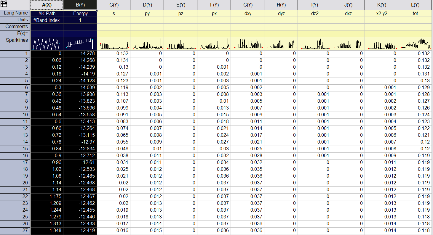
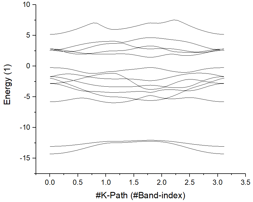
BAND.dat、BAND_REFORMATTED.dat、KLINES.dat、KLABELS、BAND_GAP文件,BAND.dat和BAND_REFORMATTED.dat文件保存了 band信息,ORIGIN 可以直接打开。BAND_REFORMATTED.dat:第一列是 K 路径的长度,单位为 Å-1,后面的列是每个波段的能量。#K-Path Energy-Level 0.000 -14.278 -13.063 -5.798 -2.813 -2.813 -1.962 -1.693 ... 0.060 -14.268 -13.058 -5.787 -2.836 -2.802 -2.055 -1.710 ... 0.120 -14.239 -13.044 -5.752 -2.906 -2.769 -2.226 -1.761 ... 0.180 -14.190 -13.021 -5.695 -3.015 -2.716 -2.416 -1.840 ... 0.240 -14.123 -12.989 -5.619 -3.157 -2.642 -2.614 -1.943 ... 0.300 -14.039 -12.948 -5.528 -3.321 -2.817 -2.551 -2.064 ... 0.360 -13.938 -12.900 -5.428 -3.496 -3.023 -2.443 -2.195 ... 0.420 -13.823 -12.846 -5.329 -3.671 -3.232 -2.333 -2.322 ... 0.480 -13.696 -12.786 -5.244 -3.830 -3.441 -2.471 -2.190 ... ...
KLABELS文件保存了带结构图上高对称点的位置:K-Label K-Coordinate in band-structure plots GAMMA 0.000 M 1.140 K 1.798 GAMMA 3.114 * Give the label for each high symmetry point in KPOINTS (KPATH.in) file. Otherwise, they will be identified as 'Undefined or XX' in KLABELS file
BAND_GAP文件保存了带隙、VBM、CBM 及其在倒易晶格处的位置信息,+-------------------------- Summary ----------------------------+ Band Character: Direct Band Gap (eV): 1.6743 Eigenvalue of VBM (eV): -0.2257 Eigenvalue of CBM (eV): 1.4485 HOMO & LUMO Bands: 9 10 Location of VBM: 0.333333 0.333333 0.000000 Location of CBM: 0.333333 0.333333 0.000000 +---------------------------------------------------------------+ NOTE: The VBM and CBM are subtracted by the Fermi Energy.
如果用户的 python 环境带有 matplotlib 模块,VASPKIT 可以自动输出
band.png图: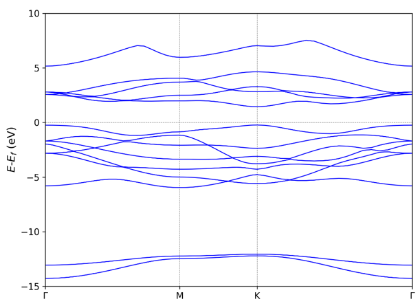
212,213,214 获取投影的带结构 :
确保 INCAR 中的 LORBIT = 10 或 LORBIT = 11 参数输出投影信息。
212) 选定原子的投影能带结构。选择投影原子:
所选原子输入数:1-4 7 8 24 或元素数:C Fe H
例如,如果要在原子 1 和 2 上绘制投影能带结构,输入 1-2:
VASPKIT 将输出两个文件:PBAND_A1.dat 和 PBAND_A2.dat。
每个文件都包含选定原子的投影信息,以及每个角动量的权重,s py pz px dxy dyz dz2 dxz x2-y2 tot。第一列是 K-path 的长度,单位为 Å-1。Second column是波段的能量。以下列是lm 轨道在该波段上的投影。最后一列是所选原子在此波段上的总投影。
213) 选定元素的投影能带结构。选择投影元素:
PBAND_S.dat 和 PBAND_Mo.dat 的格式与PBAND_A1.dat 相同。这些文件可以通过origin打开。
选择第一行和第二行,先绘制原始的 band 结构。
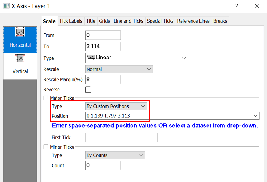
然后从 KLABELS 中找到高对称点的位置:
GAMMA              0.000
M                  1.139
K                  1.797
GAMMA              3.113
标记这些点:
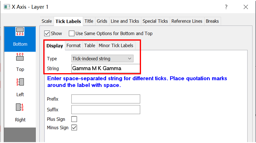
然后,调整能量范围。没有投影信息的原始波段结构显示如下。
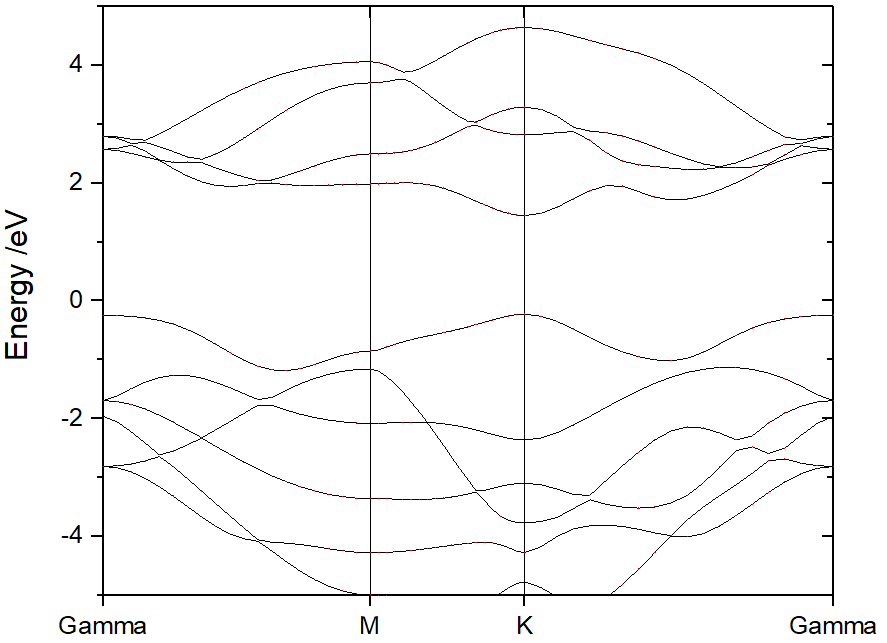
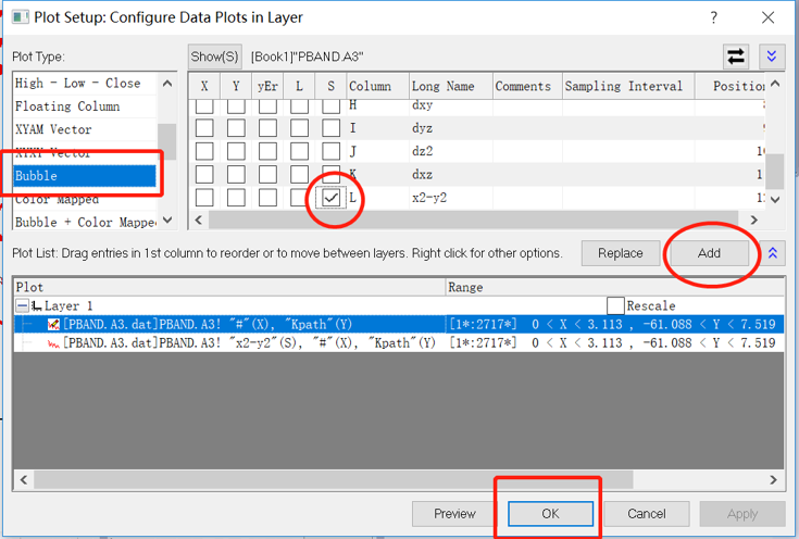
从 ORIGIN 绘图设置标签中,添加原子、元素或轨道在频带上的投影。
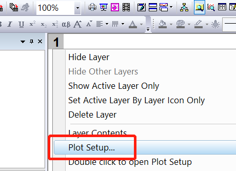
选择 Bubble tag (气泡标记),然后添加投影。单击 OK。
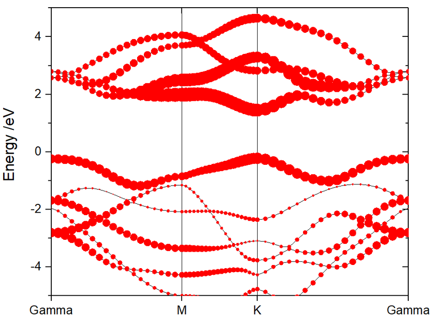
214) 选定原子的投影能带结构之和:输出 PBAND_SUM.dat 文件包括所选原子或元素的总和投影。这对于研究分层带以及比较表面带和内带非常有用。
4. 态密度(DOS)
VASPKIT 在后处理 DOS 结果方面非常强大。设置
LORBIT=10 或 11,VASP 会将每个原子的 DOS 和 l 分解或 lm 分解投影 DOS 输出到 DOSCAR 和 vasprun.xml。VASPKIT 可以提取这些信息作为用户的输入。优点:
无需下载 DOSCAR 或 vasprun.xml。直接提取 useful服务器上的 DOS。
PDOS 的选择方式很方便。元素、原子和 orbitalscan 可以根据需要选择和求和。
自动将费米能量转换为 0 eV。它可以读取 E-fermi 能量型 OUTCAR 并通过 E-fermi 移动 DOS 数据。如果不想执行 shift,只需在
~/.vaspkit中关闭它SET_FERMI_ENERGY_ZERO .FALSE. # .TRUE. or .FALSE.;
输出文件可以直接由 ORIGIN 读取,无需修改。
提取并输出 DOS 和 PDOS
选项
11用于 DOS 后处理。
| 选项 | 功能 | |
|---|---|---|
| 1 1 1 | 获取总 DOS | 输入:无。Output:TDOS.dat 包含 totalDOS;ITDOS.dat 包含整数总 DOS。旋转和下降写入一个文件中。示例:Θ-Al2O3 晶胞的总 dos |
| 1 1 2 | 将所选原子的投影 DOS 输出到单独的文件 | 输入:将元素符号和/或原子索引输入到 SUM [Total-atom:80](自由格式也可以,例如 CFe H 1-4 7 8 24)。输出:SELECTED_ATOM_LIST;PDOS_A_UP(_DW),每个选定原子的 pdos 文件;IPDOS_A_UP(_DW), 每个选定原子的 integralpdos 文件;上下旋转写入不同的文件。 |
| 1 1 3 | 将每个元素的投影 DOS 输出到单独的文件 | 输入:无。Output:P DOS_Elements_UP (_DW).dat,每个元素的 pdos 文件(每个元素的所有原子之和。IPDOS_Elements_UP(_DW).datSpin 上下旋转写入不同的文件中。 |
| 1 1 4 | 将所选原子的投影 DOS 总和输出到一个文件 | 输入:将元素符号和/或原子索引输入到 SUM [Total-atom:80](自由格式也可以,例如 CFe H 1-4 7 824)。输出:SELECTED_ATOM_LIST;PDOS_SUM_UP(_DW),用于选定原子和的 pdos 文件;IPDOS_A_UP(_DW),积分;上下旋转写入不同的文件。 |
| 1 1 5 | 将所选原子和轨道的投影 DOS 总和输出到一个文件 | 输入:将元素符号和/或原子索引输入到 SUM [Total-atom:80](自由格式也可以,例如 CFe H 1-4 7 8 24)。输入 Orbitals to Sum。哪个轨道?s py pz px dxy dyz dz2 dxz dx2f-3 ~ f3,“all”用于求和ALL。输出:PDOS_USER.datSpin 上下写入一个文件。 |
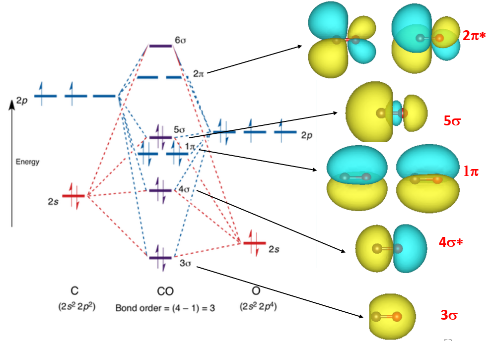
| * 示例:Ni(100) 表面 CO 吸附的 PDOS。 |
输入
/vaspkit.0.73/examples/LDOS_PDOS/Partial_DOS_of_CO_on_Ni_111_surface为每个元素运行 VASPKIT
(113) Projected Density-of-States for Each ElementVASPKIT 将输出
PDOS_Ni.dat、PDOS_C.dat和PDOS_O.dat,其中包含 Ni、C 和 O 的 PDOS 信息: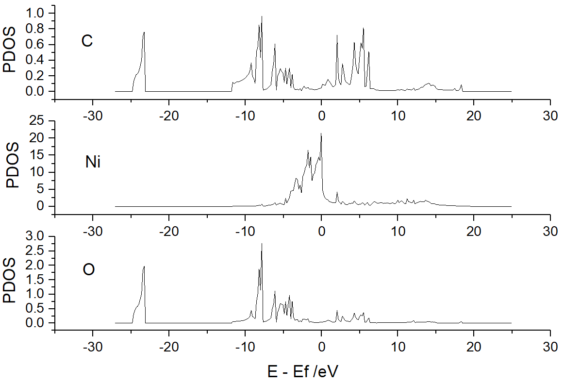
运行 VASPKIT
(114) The Sum of Projected Density-of-States for Selected Atoms,然后输入6 7将输出 CO 分子的 PDOS 总和。运行 VASPKIT
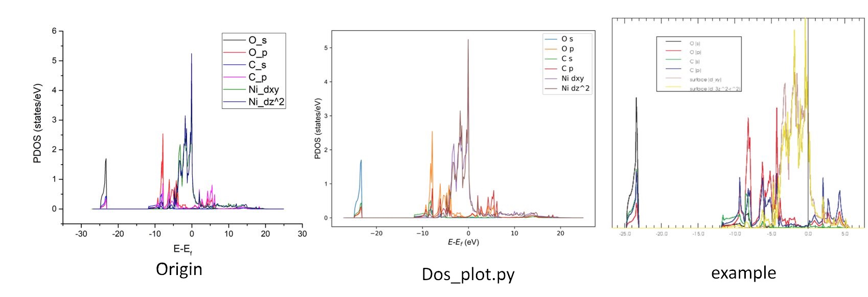
(115) The Sum of Projected DOS for Selected Atoms and orbitals。如果我们想要 O 的 s 和 p 或,C 的 s 和 p 的 p,Ni 的 d 或。Input the Symbol and/or Number of Atoms to Sum [Total-atom: 7] (Free Format is OK, e.g., C Fe H 1-4 7 8 24),Press "Enter" if you want to end e ntry! ------------>> O Input the Orbitals to Sum Which orbital? s py pz px dxy dyz dz2 dxz dx2 f-3 ~ f3, "all" for summing ALL. s ... ...
输入
O - s - O - p - C - s - C - p - Ni - d - 'Enter' - 0,然后PDOS_USER.dat文件将在此文件夹中生成,其中包含:#Energy O_s O_p C_s C_p Ni_d -27.10266 0.00000 0.00000 0.00000 0.00000 0.00000 -26.92966 0.00000 0.00000 0.00000 0.00000 0.00000 -26.75566 0.00000 0.00000 0.00000 0.00000 0.00000 -26.58266 0.00000 0.00000 0.00000 0.00000 0.00000 ... ...
Input the Symbol and/or Number of Atoms命令接受自由格式输入。您可以输入1-3 4 Ni通过选择元素 1、2、3、4 和 Ni 来累积 PDOS。Input the Orbitals to Sum命令仅支持标准输入。如果使用LORBIT=10,则只能选择 s pd f。如果使用LORBIT=11,则还支持 s py pz px dxy dyz dz2dxz dx2 f-3 f-2 f-1 f0 f1 f2。
5. 光学性质(线性光学属性)
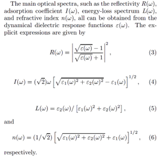
线性光学特性可以通过频率依赖性的复介电函数ε(ω) 获得
其中 ε1(ω) 和ε2(ω) 是介电函数的实部和虚部,ω 是光子频率。
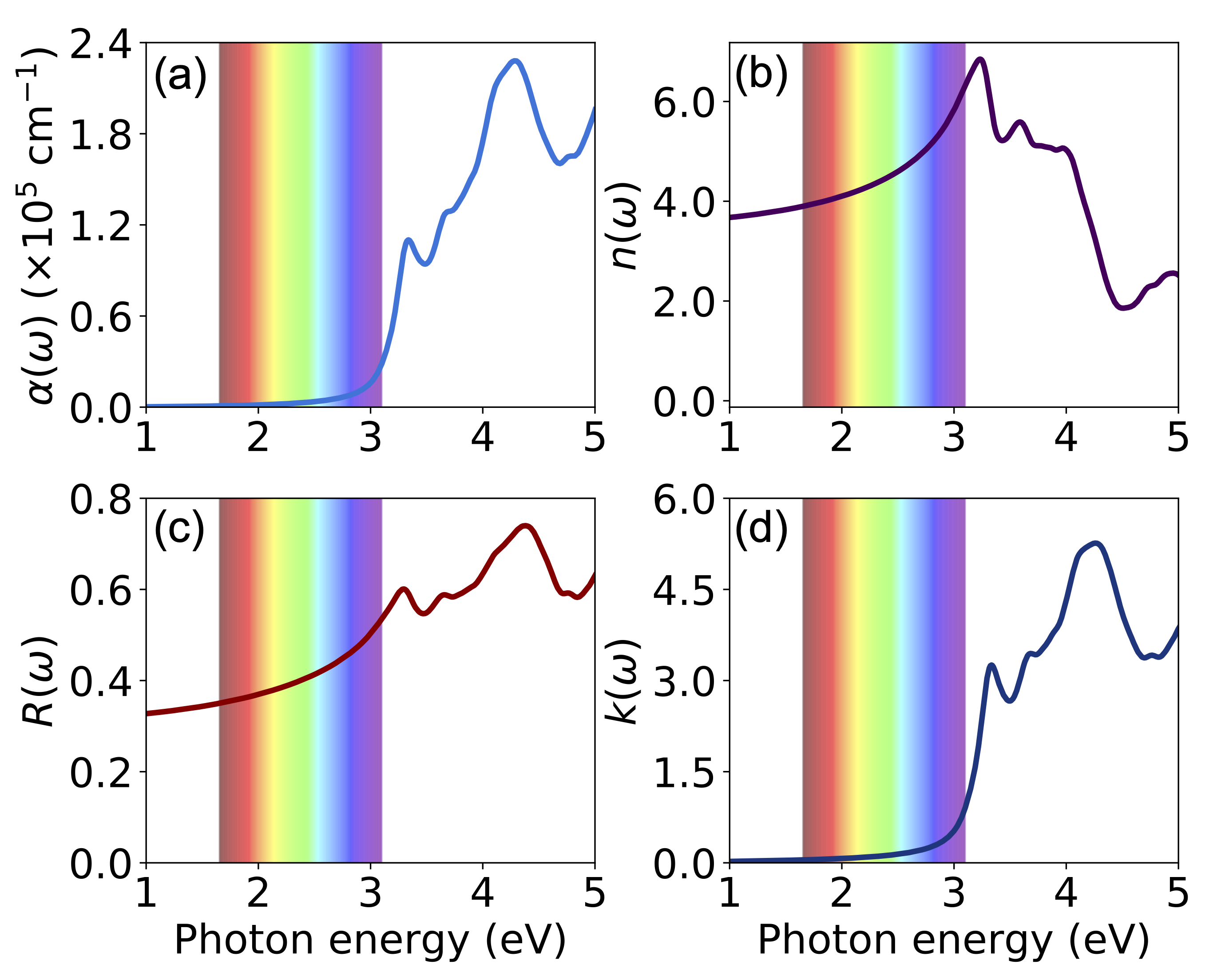
频率相关的线性光谱,例如折射率 n(ω)、消光系数 κ(ω)吸收系数 α(ω)、能量损失函数 L(ω)、反射率 R(ω) 可以从实际的 ε1(ω) 和 ε2(ω) 部分计算出来 [参见Ref. A. M. Fox, Optical Properties of Solids ]:
在 VASPKIT 版本 1.00 或更高版本中,无需运行 optical.sh 即可从第一步vasprun.xml提取图像和介电函数的实部(可选)。您可以运行 vaspkit -task 711 一次获得这些线性光谱。如果 REAL.in 和 IMAG.in 文件都不存在,程序将直接从 vasprun.xml 读取 dielectricfunction。我们以 Si 为例,计算它在 GW0+BSE 层级的光学特性,如下图所示。
创建计算文件
在完成结构优化和静态计算后,拷贝
scf文件夹为opticcp -rf ./scf ./optic
编辑
optic文件夹下INCARSYSTEM=tio2au_vacancy ISTART = 0 (Read existing wavefunction; if there) ISPIN = 1 (Non-Spin polarised DFT) # ICHARG = 11 (Non-self-consistent: GGA/LDA band structures) LREAL = Auto (Projection operators: automatic) ENCUT = 400 (Cut-off energy for plane wave basis set, in eV) PREC = Accurate (Precision level) #LWAVE = .F. (Write WAVECAR or not) #LCHARG = .F. (Write CHGCAR or not) ADDGRID= .TRUE. (Increase grid, helps GGA convergence) NPAR = 8 (Max is no. nodes, dont set for hybrids) # 相较于scf修改 NCORE = 4 - 大约等于 CPU核心数的平方根。如果你有64个核心:SQRT(64) = 8/建议的NCORE值应该在4-8之间,经验参数,需要测试。 Nwrite = 2 (Medium-level output) NBANDS = 408 # 新增(NBANDS=x x 为 OUTCAT 中 NBANDS*2, 可使用 grep 命令查询:grep NBANDS OUTCAR) LOPTICS = .TRUE. # 新增 #Electronic Relaxation ISMEAR = 0 (Gaussian smearing, metals:1) SIGMA = 0.05 (Smearing value in eV, metals:0.2) NELM = 200 (Max electronic SCF steps) NELMIN = 6 (Min electronic SCF steps) EDIFF = 1E-08 (SCF energy convergence, in eV) #Ionic Relaxation NSW = 0 (Max ionic steps) #相较于scf修改 IBRION = -1 (Algorithm: 0-MD, 1-Quasi-New, 2-CG) #相较于scf修改 ISIF = 2 (Stress/relaxation: 2-Ions, 3-Shape/Ions/V, 4-Shape/Ions) EDIFFG = -2E-02 (Ionic convergence, eV/AA) #DFT+U Calculation for Ti atoms LDAU = .TRUE. (Activate DFT+U) LDATYPE= 2 (Dudarev; only U-J matters) LDAUL = -1 2 -1 (Orbitals for each species) LDAUU = 0 6.0 0 (U for each species) LDAUJ = 0 0.5 0 (J for each species) LMAXMIX= 4 (Mixing cut-off; 4-d, 6-f) #DFT-D3 Correction IVDW = 12 (DFT-D3BJ method of method with no damping)
其他3个文件保持与
scf相同,然后提交任务。计算完成后,可查看
OUTCAR文件,有计算得出介电常数(Dielectric constant)的实部和虚部。frequency dependent IMAGINARY DIELECTRIC FUNCTION E(ev) X Y Z XY YZ ZX frequency dependent REAL DIELECTRIC FUNCTION E(ev) X Y Z XY YZ ZX
使用vaspkit程序对计算结果进行处理
光学数据处理:
输入命令
optic产生REAL.IN和IMAG.IN文件。或者依次输入命令vaspkit和71,屏幕显示如下:71 ======================= Optical Options ========================= 710) Linear Optical Spectrums for Two-Dimensional Semiconductors 711) Linear Optical Spectrums for Bulk Semiconductors 713) Transition Dipole Moment from WAVECAR file 714) Dipole Moment Elements from WAVEDER file 716) Total Joint Density of States 717) Partial Joint Density of States between Two Bands 719) Spectroscopic Limited Maximum Efficiency 0) Quit 9) Back ------------>> 711 +---------------------------- Tip ------------------------------+ | See an example in vaspkit/examples/Si_bse_optical. | | This utility is NOT suitable for low-dimensional materials. | +---------------------------------------------------------------+ ===================== Energy Unit =============================== Which unit of energy would you like to use? 1) eV 2) nm 3) THz 4) cm^-1 ------------>> 1 -->> (01) Reading Input Parameters From INCAR File. -->> (02) Reading Dielectric Function From vasprun.xml File. -->> (03) Written REAL.in and IMAG.in Files. -->> (04) Reading IMAG.in and REAL.in Files... -->> (05) Written Linear Optical Files Succesfully!
输出文件
ABSORB.dat,REFRACTIVE.dat,REFLECTIVITY.dat,EXTINCTION.dat和ENERGYLOSSSPECTRUM.dat,依次为absorption coefficient,refractive coefficient,reflectivity coefficient,extinction coefficient and energy-loss function。导出使用Origin作图即可。附:相关光学性质计算公式
相关参考
关于LOPTICS参数的介绍
LOPTICS = .TRUE. | .FALSE.
默认:LOPTICS = .FALSE.
描述:LOPTICS =.TRUE. 在确定电子基态后计算频率相关的介电矩阵。
虚部由空状态的求和使用以下方程确定:
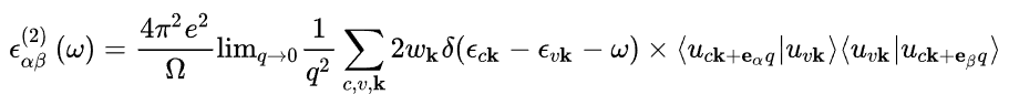
在这里,指标_c_和_v_分别指传导带和价带状态,而_u__c_k 是 k 点处轨道的晶胞周期部分。介电张量 ε(1) 的实部通过通常的克拉默斯 - 克勒尼希变换获得。
其中,_P_表示主值。Gajdoš等人的论文中详细解释了该方法(见公式 15、29 和 30)。等。[1]0复数位移 η 由参数CSHIFT决定。
请注意,在这种近似下,局部场效应,即电势的晶胞周期性部分的变化被忽略了。这些可以使用已实现的密度泛函微扰理论(LEPSILON=.TRUE.)或 GW 例程进行评估。
使用 LOPTICS=.TRUE. 所选的方法需要相当数量的空导带态。通常只有在相对于 VASP 默认值在INCAR文件中将参数NBANDS大致增加一倍或两倍时才能获得合理的结果。此外,需要强调的是,即使对于HF 和屏蔽交换类型计算以及混合泛函,该例程也能正常工作。在这种情况下,使用有限差分来确定哈密顿量相对于 k 的导数。
请注意,频率网格点的数量由参数 NEDOS 决定。在许多情况下,最好从其默认值显著增加此参数。强烈建议使用 NEDOS=2000 左右的值。
VASP 拥有多个其他例程来计算频率相关的介电函数。具体而言,可以使用ALGO=TDHF(卡西达 /BSE 计算)、ALGO=GW(GW 计算)和ALGO=TIMEEV(时间演化:应用一个微扰并跟踪感应偶极子)。与 LOPTICS=.TRUE. 相比,所有这些例程都具有包含独立粒子近似之外的效应的优势,然而,它们通常也比 LOPTICS=.TRUE. 昂贵得多。
Spectral broadening 光谱展宽:用 LOPTICS 计算的介电函数包括由于涂抹方法ISMEAR引起的展宽以及由于克喇末 - 克勒尼希变换中的复位移引起的洛伦兹展宽。例如,LOPTICS=.TRUE. 和ISMEAR=0 的组合产生了由宽度为SIGMA的高斯函数和宽度为CSHIFT的洛伦兹函数展宽的介电函数。为了避免同时使用两种不同的展宽方法而仅包含洛伦兹展宽,应将SIGMA设置为比CSHIFT小得多的值。
6. 跃迁偶极矩
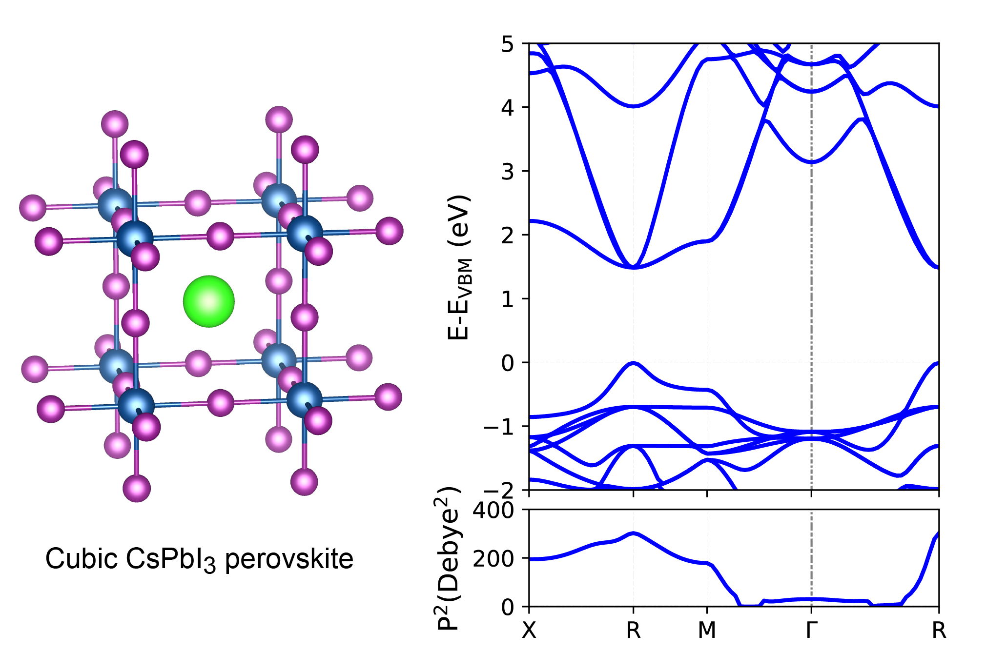
跃迁偶极矩 (TDM) 或过渡矩,通常表示初始状态 a 和最终状态 b 之间的过渡,是与两种状态之间的过渡相关的电偶极矩。通常,TDM 是一个复矢量,其中包括与两种状态相关的相位因子。它的方向给出了跃迁的极化,这决定了系统将如何与给定极化的电磁波相互作用,而幅度的平方给出了由于系统内电荷分布而产生的相互作用的强度。过渡偶极矩的 SI 单位是库仑米 (Cm);一个更方便的单位是 Debye (D)。价带和导带之间的转换概率由计算出的 TDM 平方和(以 Debey2 为单位)来显示。
我们以立方 CsPbI3 钙钛矿相为例,并给出了 PBE 计算的能带结构和相应的 TDM,如下图所示。该系统共有 44 个价电子。接下来,我们计算从最高价带(能带指数 22)到最低导带(能带指数 23)的过渡偶极矩的平方。结果发现与之前的发现非常吻合(参见 参考文献 J. Phys. Chem. Lett . 2017, 8, 2999−3007)。
计算过程与能带结构计算非常相似,除了设置 LWAVE=.TRUE. 在 INCAR 文件中。有关这些计算的更多详细信息,请参阅 vaspkit/examples/tdm。
 ------------>>
71
 ============================ Optical Options ====================
 1)   Linear Optical Spectrums
 2)   Transition Dipole Moment at Single kpoint
 3)   Transition Dipole Moment for DFT Band-Structure

 4)   Quit
 5)   Back
 ------------>>
713
 +-------------------------- Warm Tips --------------------------+
            See an example in vaspkit/examples/tdm.
 ONLY Support KPOINTS created by VASPKIT for hybrid bandstructure.
 +---------------------------------------------------------------+
 ======================= Band-Structure Mode ====================
 1) DFT Band-Structure Calculation
 2) Hybrid-DFT Band-Structure Calculation

 ------------->>
1
 Please input TWO bands separated by spaces.
 (e.g., 4 5 means to get TDM between 4 and 5 bands at all kpts)

 ------------>>
22 23
 +-------------------------- Warm Tips --------------------------+
   Current Version Only Support the Stardard Version of VASP code.
 +---------------------------------------------------------------+
  -->> (01) Reading the header information in WAVECAR file...
 +--------------------- WAVECAR Header --------------------------+
 SPIN =    1
 NKPTS =   80
 NBANDS =  36
 ENCUT =   400.00
 Coefficients Precision: Complex*8
 Maximum number of G values: GX =   11, GY =   11, GZ =   11
 Estimated maximum number of plane-waves:    5575
 +---------------------------------------------------------------+
  -->> (02) Start to read WAVECAR file, take your time ^.^
            Percentage complete:  25.0%
            Percentage complete:  50.0%
            Percentage complete:  75.0%
            Percentage complete: 100.0%
  -->> (03) Reading K-Paths From KPOINTS File...
  -->> (04) Start to calculate Transition Dipole Moment...
            Percentage complete:  25.0%
            Percentage complete:  50.0%
            Percentage complete:  75.0%
            Percentage complete: 100.0%
  -->> (05) Written TDM.dat File!
如果要计算 single k-point处两个状态之间的 TDM 平方。只需使用任务 712 运行 vaspkit,例如,
71
 ============================ Optical Options ====================
 1)   Linear Optical Spectrums
 2)   Transition Dipole Moment at Single kpoint
 3)   Transition Dipole Moment for DFT Band-Structure

 4)   Quit
 5)   Back
 ------------>>
712
 +-------------------------- Warm Tips --------------------------+
             See an example in vaspkit/examples/tdm.
           Please Set LWAVE= .TRUE. in the INCAR file.
 +---------------------------------------------------------------+
 Input ONE kpoint and TWO bands separated by spaces.
 (e.g., 1 4 5 means to get TDM between 4 and 5 band at 1st kpt)

 ------------>>
1 22 23
 +-------------------------- Warm Tips --------------------------+
   Current Version Only Support the Stardard Version of VASP code.
 +---------------------------------------------------------------+
  -->> (01) Reading the header information in WAVECAR file...
 +--------------------- WAVECAR Header --------------------------+
 SPIN =    1
 NKPTS =   80
 NBANDS =  36
 ENCUT =   400.00
 Coefficients Precision: Complex*8
 Maximum number of G values: GX =   11, GY =   11, GZ =   11
 Estimated maximum number of plane-waves:    5575
 +---------------------------------------------------------------+
 Square of TDM (Debye^2):  X           Y           Z        Total
                         0.000     201.617       0.000     201.617
显然,立方相 CsPbI₃在 X 点处的跃迁偶极矩(Transition Dipole Moment,TDM)总平方值为 201.62 德拜 。
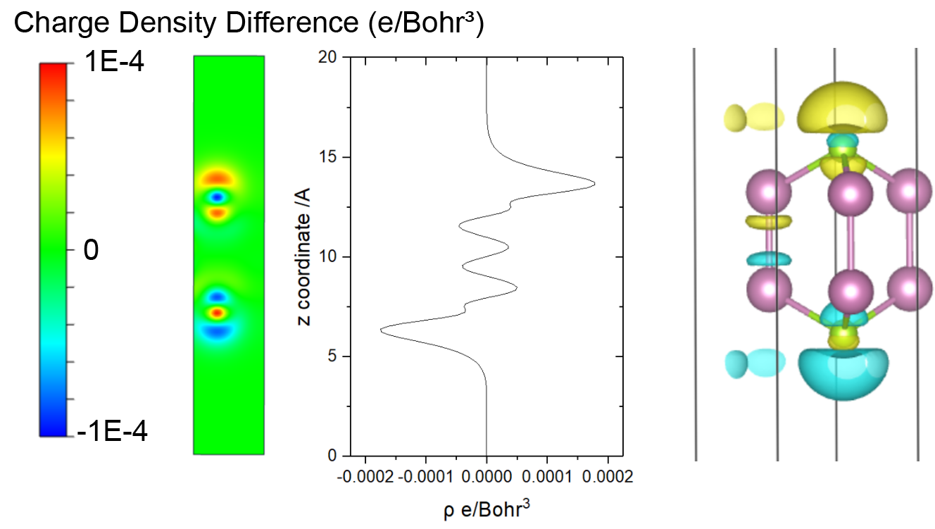
7. 电荷密度差(CDD)
示例:两个片段的电荷密度差异
优化 CO/Ni(100) 的结构
分别对 Ni(100) 和 CO进行单点自洽计算。 注意 :CO 和 Ni(100) 片段的原子位置应取自优化的 CO/Ni(100) 片段,不要优化 CO 和 Ni(100) 片段!
运行 VASPKIT
314。分别输入三个 CHGCAR 的路径:314 ======================= File Options ============================ Input the Names of Charge/Potential Files with Space: (e.g., to get AB-A-B, type: ~/AB/CHGCAR ./A/CHGCAR ../B/CHGCAR) (e.g., to get A-B, type: ~/A/CHGCAR ./B/CHGCAR) ------------>> ./CHGCAR ./co/CHGCAR ./slab/CHGCAR -->> (01) Reading Structural Parameters from ./CHGCAR File... -->> (02) Reading Charge Density From ./CHGCAR File... -->> (03) Reading Structural Parameters from ./co/CHGCAR File... -->> (04) Reading Charge Density From ./co/CHGCAR File... -->> (05) Reading Structural Parameters from ./slab/CHGCAR File... -->> (06) Reading Charge Density From ./slab/CHGCAR File... -->> (07) Written CHGDIFF.vasp File!
输出 CHGDIFF.vasp 也是一个可由 VESTA 打开的网格。
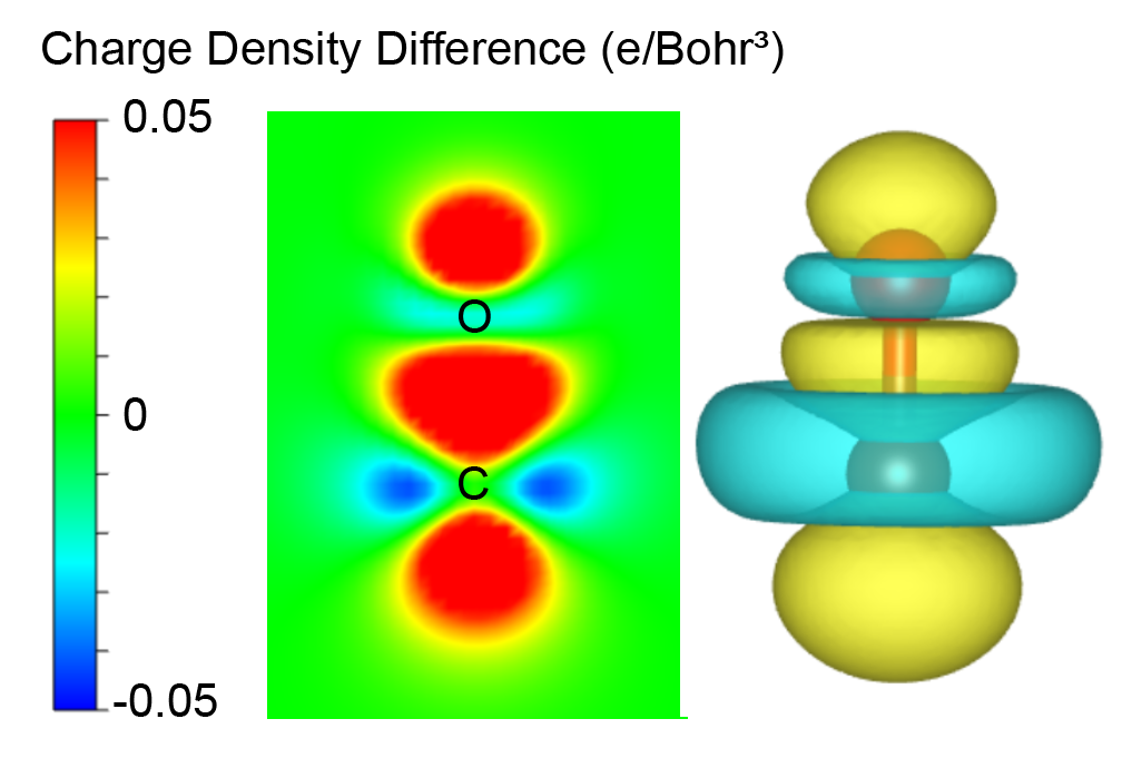
示例:CO的变形电荷密度
对 CO 分子进行自洽计算。
创建一个新文件夹,进行非自洽计算以输出原子电荷密度的叠加。
运行 VASPKIT
314分别输入两个 CHGCAR 的路径。314 ======================= File Options ============================ Input the Names of Charge/Potential Files with Space: (e.g., to get AB-A-B, type: ~/AB/CHGCAR ./A/CHGCAR ../B/CHGCAR) (e.g., to get A-B, type: ~/A/CHGCAR ./B/CHGCAR) ------------>> ./CHGCAR ./deform/CHGCAR -->> (01) Reading Structural Parameters from ./CHGCAR File... -->> (02) Reading Charge Density From ./CHGCAR File... -->> (03) Reading Structural Parameters from ./deform/CHGCAR File... -->> (04) Reading Charge Density From ./deform/CHGCAR File... -->> (05) Written CHGDIFF.vasp File!
输出 CHGDIFF.vasp 文件,然后通过 VESTA 打开它。
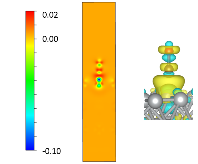
示例:InSe 的电荷密度与电场的差异
优化了无外部电场的 InSe 结构。
基于 optimized structure 进行自洽的单点计算。
EFIELD = 0.05
IDIPOL = 3
LDIPOL = .TRUE.
# EFIELD 控制施加的电动场的大小,单位为 eV/Å。
运行 VASPKIT
314进行CDD计算。输出 CHGDIFF.vasp 文件,然后通过 VESTA 打开它。
8. 实空间中的 WaveFunction 可视化
VASPKIT可以从WAVECAR文件中提取Kohn-Sham(KS)轨道的平面波系数,并输出实空间波函数。用户需要输入要绘制的 K 点和要绘制的波段。
注意:现在,VASPKIT 一次只能输出指定的 1K 点和一个波段的波函数。要对几个 K 点求和或设置能量范围,VASP 中的部分电荷密度计算就可以了。
示例:CO 分子的 WaveFunction
检查带结构或
IBZKPT文件以检查您要绘制哪个 K 点?对于 CO 分子计算,只有一个 Gamma 点。所以输入1Which K-POINT do you want to plot? (1<= ikpt <=1) ------------>> 1
检查带结构或
EIGENVAL文件以检查您要绘制的带?EIGENVAL 文件显示如下。五列分别是: 1, band number; 2, spin up band energy; 3, spin down band energy; 4, spin up occupation number; 5, spin down occupation number.如果要检查HOMO和LUMO或VBM和CBM,依次选择波段5、6、7。
511
+-------------------------- Warm Tips --------------------------+
    Open Real-Space WaveFunction Files with VESTA/VMD Package.
+---------------------------------------------------------------+
Which K-POINT do you want to plot? (1<= ikpt <=1)

------------>>
1
Which BAND do you want to plot? (1<= iband <=36)

------------>>
5
+-------------------------- Warm Tips --------------------------+
  Current Version Only Support the Stardard Version of VASP code.
+---------------------------------------------------------------+
  -->> (01) Reading the header information in WAVECAR file...
+--------------------- WAVECAR Header --------------------------+
SPIN =    2
NKPTS =    1
NBANDS =  36
ENCUT =   400.00
Coefficients Precision: Complex*8
Maximum number of G values: GX =   25, GY =   25, GZ =   25
Estimated maximum number of plane-waves:   65450
+---------------------------------------------------------------+
  -->> (02) Start to Post-Process Wavefunctions...
  -->> (03) Reading Structural Parameters from POSCAR File...
  -->> (04) Written RWAV_B0005_K0001_UP.vasp File!
  -->> (05) Written IWAV_B0005_K0001_UP.vasp File!
  -->> (06) Written RWAV_B0005_K0001_DW.vasp File!
  -->> (07) Written IWAV_B0005_K0001_DW.vasp File!

Note: Now, VASPKIT can only output wavefunction for specified one K points and one band at one time. To sum several K points or seting the energy range, VASP partial charge calculation can do it.
输出文件格式为 VASP 网格文件,与 CHGCAR 相同,可通过 VESTA 打开。
RWAV是波函数的实部,IWAV是波函数的虚部。通常,我们只需要绘制和分析实际部分,B0005是 IBZKPT 文件中的波段数,K0001是 K 点数。Spin up 和 Spin down 分别输出。显示RWAV_B0005_K0001_UP.vasp、RWAV_B0006_K0001_UP.vasp和RWAV_B0007_K0001_UP.vasp…文件。
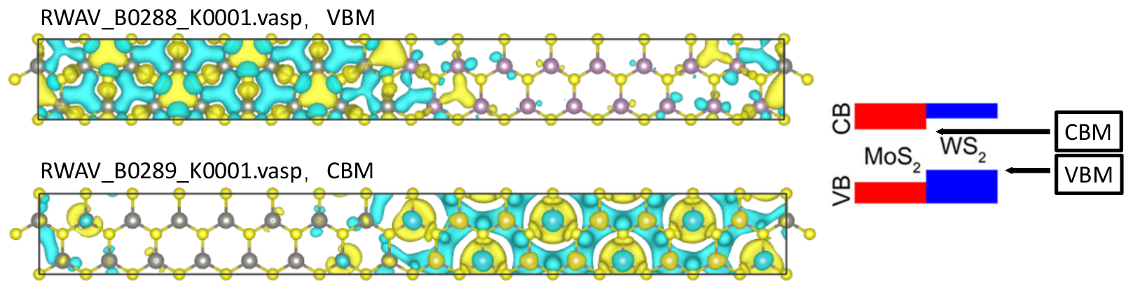
示例:MoS2/WS2 异质结的 WaveFunction
检查
IBZKPT文件和EIGENVAL文件。EIGENVAL显示 Gamma 的 VBM 和 CBM 为:... 287 -2.799024 1.000000 288 -2.799005 1.000000 289 -0.201544 0.000000 290 -0.201541 0.000000 ...
提取 Gamma 点处的
288和289波段。运行 VASPKIT,输入511-1-288和511-1-289。打开RWAV文件。
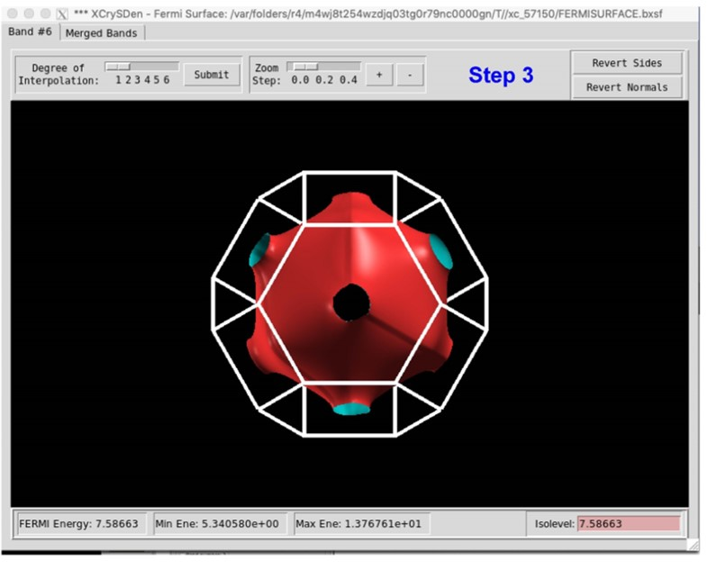
9. 费米面
在凝聚态物理学中,费米表面是在零温度下将占用带与未占用带分开的表面互易空间。费米表面的形状来自晶格的周期性和对称性以及电子能带的占据。
准备 FCC Cu 的优化 POSCAR。注意它必须是原始单元。
运行 VASPKIT 并输入
261命令以生成用于计算费米表面的 KPOINTS 和 POTCAR 文件。------------>> 261 +-------------------------- Warm Tips --------------------------+ \* Accuracy Levels: (1) Medium: 0.02~0.01; (2) Fine: < 0.01; \* 0.01 is Generally Precise Enough! +---------------------------------------------------------------+ Input KPT-Resolved Value (unit: 2*PI/Angstrom): ------------>> 0.008 -->> (1) Reading Structural Parameters from POSCAR File... -->> (2) Written KPOINTS File!
提交 VASP 作业。
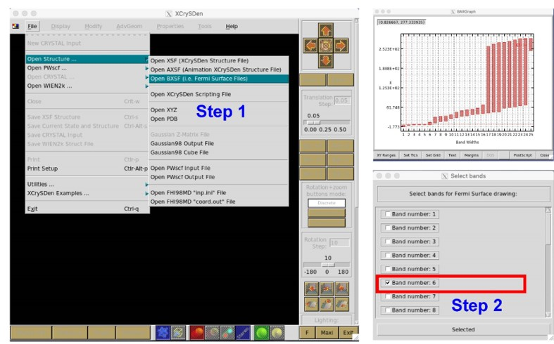
VASP 计算完成后,再次运行 VASPKIT,输入
262命令,生成包含费米表面数据的 FERMISURFACE.bxsf 文件。------------>> 262 -->> (1) Reading Input Parameters From INCAR File... -->> (2) Reading Structural Parameters from POSCAR File... -->> (3) Reading Fermi-Level From DOSCAR File... ooooooooo The Fermi Energy will be set to zero eV oooooooooooooooo -->> (4) Reading Energy-Levels From EIGENVAL File... -->> (5) Written FERMISURFACE.bxsf File!
运行 XcrySDen 软件并按照以下步骤作。第五个带穿过费米表面,所以我们选择波段数 5,然后点击 Selected,然后得到 Cu 的费米表面。
10. 后记:vaspkit 的安装与使用
将已下载的
VASPKIT导入linux服务器,安装步骤:tar -zvxf vaspkit.*.tar.gz cd vaspkit.* ./setup.sh # Note that the formats of POSCAR, CONCAR and CHGCAR files in VASP.5.x are slightly different from those in VASP.4.x. Please set the vasp5=.false. in the src/module.f90 file if you use VASP.4.x
设置环境变量:
export PATH=/opt/apps/tools/vaspkit.1.5.1/bin:${PATH}
alias optic="/opt/apps/tools/vaspkit.1.5.1/examples/Si_BSE_optical/optical.sh"
alias vaspkit="/opt/apps/tools/vaspkit.1.5.1/bin/vaspkit"
# You need to preparetheREAL.IN anIMAG.IN files which include the real and imaginary parts of frequencydependent complex dielectric function. There is a bash scriptoptics.sh as a reference in the vaspkit.*/examples/optic/ could help you to prepare the real.in and imag.in files.
11. Computational 2D Semiconductor Database
通过高通量第一性原理计算,根据能量、热力学、机械、动力学和热稳定性标准,从近 1000 个单层中筛选出约 270 个二维非磁性半导体。研究者展示了所有满足我们标准的候选者的计算结果,包括晶格常数、形成能、杨氏模量、泊松比、剪切模量、带隙、带结构、电离能和电子亲和力。The data can be browsed online: Browse data